WIXLIB

124type of rainfall simulator is the most common device used in semi-arid areas in Europe,125especially in Spain, and major differences typically occur in pumps, nozzles and applied126intensities. Duration of all simulators is adjustable, only the WA-simulator is limited to three127min, due to its compact design.128129Table 1130The main characteristics of small scale portable rainfall simulators tested (ranked in order of plot size).Plot size[m²]Plot designFallingheight [m]Nozzle / DropformersWater sourceDetailsTU1.0001 m x 1 m,rectangular3.43Lechler 460.788.30Electric pressure pump (driven bypower generator)Iserloh et al. (2013)CO0.7001 m x 0.7 m,rectangular2.30Veejet 80.150Electric pressure pump (driven bypower generator)Alves Sobrinho et al. (2008)BA0.7001.34 m x 1.0 m x0.3 m, trapezoid1.10Spraying Systems3/8 HH 20W SQElectric pressure pump (driven bypower generator)Hikel et al. (2013); Iserloh et al.(2013)GR0.2500.5 m x 0.5 m,rectangular1.504900 capillaries per m²Electric peristaltic pump (driven bypower generator) Mariotte‘s bottleFernández-Gálvez et al. (2008)AL0.283round2.00Hardi 4680-10EGasoline engine driven pressurepumpe.g. Li et al. (2011)MA0.283round2.00Hardi 1553-20Electric pressure pump (driven bypower generator)e.g. Martínez-Murillo and RuizSinoga (2007)MU0.283round2.00Lechler 402.608.30Gasoline engine driven pressurepumpMartínez-Mena et al. (2001b)TR0.283round2.00Lechler 460.608.30Gasoline engine driven pump orelectrical pump (driven by battery)Iserloh et al. (2012, 2013)ZAC0.283round2.22Lechler 460.688.30Gasoline engine driven pressurepumpNadal-Romero and Regüés(2009); Nadal-Romero et al.(2011)VA0.246round2.00Hardi 1553 12Gasoline engine driven pump orelectrical pump (driven by battery)Cerdà et al. (1997); Iserloh et al.(2013)ZAU0.212round2.18Lechler 460.688.30Gasoline engine driven pressurepumpIserloh et al. (2013); León et al.(2013)LR0.160round2.50Lechler 460.608.17Gasoline engine driven pressurepumpArnaez et al. (2007)WA0.1590.24 m x 0.24 m,rectangular0.4049 capillariesCylindrical reservoir over capillariesIserloh et al. (2013); Kamphorst(1987)ID1311322.2 Methods for evaluating rainfall characteristics133a) Drop size distribution and drop fall velocities134The Thies Laser Precipitation Monitor (LPM) was used for analysing the DSD and drop fall135velocities. LPM measures the amount and intensity of rainfall and determines rain-drop size136and velocity as the drops fall through a laser beam (area of 46 cm2 (23 x 2 cm)). It registers137individual drops with diameters ranging from 0.16 mm to 8 mm, and fall velocities ranging138from 0.2 m s-1 to 20 m s-1, up to a maximum intensity of 250 mm h-1 (Thies, 2004). A more139detailed description of the LPM is given in Angulo-Martínez et al. (2012), Fister et al. (2012),5

140King et al. (2010) and Scholten et al. (2011). Because the LPM records only drop size and drop141velocity classes, we used the mean value of each class to calculate kinetic energy,142momentum and median volumetric drop diameter (d50).143b) Spatial rainfall distribution144In order to generate quantitative information about the homogeneity and the reproducibility of145rainfall, small rainfall collectors were used to measure the spatial rainfall distribution. The146entire test plot was covered by collectors: square ones (56 cm²; in case of Basel: 100 cm²)147for square plots and round collectors (20 cm²) for round plots (Fig 2).1481492.3 Test procedure150A standardized test procedure was developed and performed with the simulators.151Prior to each test sequence, rainfall intensity was calibrated using the method generally152applied by each group to maintain the customary rainfall conditions of their experimental153work. TR and VA used a calibration plate covering the whole plot, TU used the LPM154technique, and the remaining groups used rain collectors.155Water discharge of nozzles was determined using the volumetric method.156In order to analyse drop spectra with the LPM, five representative positions within the total157plot area were chosen (Fig. 2). At each position, five replications at one minute measurement158intervals were performed (except the WA-simulator whose design allows only a maximum159duration of three minutes). Due to the bodywork of the LPM, the measurement height is16015 cm above ground.161Exposure time of collectors to rainfall during each replicate experiment was five min, and a162total of three repetitions were undertaken. The individual collectors were weighed to163determine spatial variations in the mass, and hence the volume of water at each location164within the plot. The results were calculated as equivalent intensity values (mm h-1) and165spatially displayed. The measurement of rainfall distribution of the WA-simulator was not166possible due to the compact construction of the simulator.6

Fig. 1. The small-scale portable rainfall simulators from a) Tübingen(TU), b) Cordoba (CO), c) Basel (BA), d) Granada (GR), e) Almeria(AL), f) Malaga (MA), g) Murcia (MU), h) Trier (TR), i) ZaragozaCSIC (ZAC), j) Valencia (VA), k) Zaragoza-University (ZAU), l) LaRioja (LR) and m) Wageningen (WA).1677

168169Fig. 2. Test set-up: a) Tübingen (TU), b) Cordoba (CO), c) Basel (BA), d) Granada (GR), e) Almeria170(AL), Malaga (MA), Murcia (MU), Trier (TR), Zaragoza-CSIC (ZAC), Valencia (VA) and Zaragoza-171University (ZAU), f) La Rioja (LR) and g) Wageningen (WA). LPM Laser Precipitation Monitor.1721732.4. Further calculations174a) Rainfall kinetic energy and momentum175Rainfall kinetic energy was calculated using equations from Fornis et al. (2005). These176equations were provided relating to the development of the Disdrometer RD-80 (Disdromet177Ltd, Basel, Switzerland, 2001) and are optimally applicable for the LPM by Thies. In order to8

178compute the rate of kinetic energy expenditure ( KE R , J m-2 h-1) for every 1-min period, the179following equation was used:180 1 3600 1 203KE R 6 ni Di vDi1210tA i 1 181where A 0.0046 m2 is the sampling area of the LPM, ni the number of drops of diameter182Di ; vDi the measured fall velocity of drop with diameter Di and t 60 s.183The kinetic energy per unit area and unit depth of rainfall, KE (J m-2 mm-1) was calculated184using equation (2):185 KE R KE I 186where I is the rainfall intensity (mm h-1) measured with the LPM.187Brodie and Rosewell (2007) concluded that key processes of particle wash-off due to rainfall188are slightly more dependent on momentum (M) than on KE, therefore momentum was189calculated following their approach. The calculations in equation (3) were made on the basis190that the momentum M (kg m s-1) of an individual raindrop of diameter Dn is:191M n 10 3 mn v Fn192where mn is mass (g) of Dn raindrop, v Fn is terminal fall velocity (m s-1) of Dn raindrop in still193air.194v Fn is measured by the LPM, the mass, mn , must be calculated (Eq. 4), and the drop volume195Vn (mm³) is to be determined (Eq. 5), while it is calculated from the measured drop196diameters Dn .197mn 10 3 Vn198Vn 6Dn32(1)(2)(3)(4)(5)1992002019

202b) Median volumetric drop diameter203The median volumetric drop diameter (d50) was calculated from the percentage total mass of204raindrops in each size class according to Hudson (1995) and Clarke and Walsh (2007). For the205calculation, the volumes of spherical drops have been assumed.206c) Uniform Coefficient and spatial rainfall variability207In order to compare results between different simulators, the mean Christiansen Uniformity208(CU) coefficient (Christiansen, 1942) was calculated using equation (6).nCU (1 209n210where xi 1i xi 1i xx*n)(6) x is the sum of the absolute deviations from mean water amount of all rain211collectors [ml], xi is individual water amount per rain collector [ml], x is the arithmetic mean212of applied water amount per rain collector [ml] and n is the total number of rain collectors.213For the characterisation of spatial rainfall variability, the deviation from the mean was214calculated for each collector based on the three replicate tests performed for each rainfall215simulator. The deviation was then normalised by the mean rainfall intensity of the respective216cell to compute a quantitative measure for the spatial reproducibility of simulated rainfall.2172183. Results and discussion219The main rainfall characteristics for each simulator are presented in Table 2. The rainfall220simulators of the participating institutes produced a broad range of intensities, from 37 mm h-2211222intensity, the plot size and the size of nozzle used (e.g. due to different spray angles and223applied water pressure). The results ranged from 0.49 L min-1 for AL and VA, to 3.24 L min-1224for TU. Water efficiency showed a broad data range from 4.2 % (LR: large spray angle, high225water pressure) to 49.3% (AL: small spray angle, low water pressure). Particularly for those226in situ rainfall simulator studies in (semi-) arid areas with limited water availability, water227consumption should be as low and used as efficiently as possible.(MA) to 360 mm h-1 (WA). Total water consumption per min depends on the applied10

228Table 2229Main results of simulated rainfall characteristics for each rainfall simulator: water consumption, water230efficiency, mean Intensity [I], Christiansen Uniformity [CU], mean spatial variability (average deviation231from mean) of rainfall distribution, mean drop number [n], median volumetric drop diameter [d50], mean232kinetic energy expenditure [KER], mean kinetic energy per unit area per unit depth of rainfall [KE] and233mean momentum [M].WaterconsumptionID[L min-1][%]I[mm h-1]CU[%]Spatialvariabilityn [min-1][%]d50KERKEM[mm][J m-2 h-1][J m-2 mm-1][kg m 9650.320.0917WA234WaterefficiencyaNot measured235236Drop spectra237The mean drop size and fall velocity measurements with the LPM are listed in Fig. 3. The238major similarity is that maximum drop numbers are attained within the two smallest drop size239classes 1 mm (Fig. 3 and Fig. 4): in all cases, except TU and WA, 1000 drops per min240were only measured in those classes 1 mm. TU also reached 1059 drops in the drop size241class 1.0-1.49 mm; the drop amounts of WA are lower than 1000 drops per min for all drop242size classes. Amounts of drops 1 mm were generally much lower than that of 1 mm: max.243833 drops per min (ZAU) were measured in the drops size class 1.0-1.49 mm and a max. of11

244554 drops per min (AL) was detected for sizes 1.5 mm. The highest number of drops per245min 2.0 mm was measured for WA (320 drops per min). More than 100 drops per min246 3.0 mm were only produced by the two capillary-type simulators GR (166 drops per min)247and WA (153 drops per min).248The data also show that the fall velocity of bigger drops is lower due to the general physical249restriction of low drop fall heights (Fig. 3). During all simulations, 90% or more of the250measured drops were slower than 3.4 m s-1. Only TU (237 drops), CO (321 drops) and GR251(158 drops) generated more than 100 drops per min with fall velocities 5 m s-1. Drops252 5.8 m s-1 were rarely measured. A few drops with velocities around 9 m s-1 were measured253during simulations of CO, because the special water application unit in the simulator is able254to accelerate bigger drops to higher fall velocities. The velocities of smaller drops ( 1 mm)255generated by the simulators were often similar to that expected for natural drops, as256indicated by Atlas et al. (1973) and Mätzler (2002), for vertical rainfall in calm conditions. In two257cases (TU and TR), more than 100 larger drops (1.0-1.49 mm) per min were accelerated to258expected natural velocities.259By examining single rainfall simulators, four groups can be distinguished. During the runs of260BA, ZAC, ZAU and LR, hardly any big drops ( 2.5 mm) were measured. The simulators from261TU, MA, MU, TR and VA produced drops 2.5 mm, but this was much less than the capillary-262type simulators from GR and ZAU. The simulators from CO and AL also generated drops263 2.5 mm but reached higher velocities than GR and ZAU.264Unfortunately, determining exact d50 values for volumetric drop diameter was not possible265with the LPM for two reasons. As mentioned above, the device records only size classes and266not actual drop sizes, besides the fact that only drop diameters are registered. We assumed267a circular form of the falling drops for our calculations (Fister et al., 2011). Nevertheless,268calculation of d50 values represents the best possible option for comparison with other rainfall269simulators (Fister et al., 2012; Hudson, 1995). Hence, the lowest d50 value of the 13 simulators270was 0.375-0.750 mm (LR), and the highest was 5.5-6.5 mm (WA) (Table 2).12

271Most studies lack accuracy concerning calculated kinetic energy of simulated rainfall (Clarke272and Walsh, 2007): the values are predominantly calculated from intensities only, based on the273assumption that diameters and/or velocities from natural rainfall apply for simulated rainfall,274too. Considering the general physical restrictions of simulated rainfall (e.g. fall height), we275therefore assume, that most of the published data overestimate real values of kinetic energy.276The KE values calculated in this study were maximal 56 % and minimal 3 % of the KE277calculated with the three of the most commonly used equations for determining natural278rainfall of equal intensities (van Dijk et al., 2002; Morgan et al., 1998; Wischmeier and Smith,2791978). Only the WA produced rainfall with a KE that was greater than that calculated for280natural rainfall (up to 77 % more than calculated with each of the three mentioned281equations). The high KE of the WA-simulator was caused by the specific characteristics (very282short test duration with large, high-energy drops as described in Iserloh et al. (2013) and283Kamphorst (1987).284The calculated momentums of simulated rainfalls ranged from 0.0042 kg m2 s-1 for LR up to2850.0917 kg m2 s-1 for WA. As mentioned above, some researchers concluded that key286processes of particle wash off due to rainfall are slightly more dependent on momentum than287on KE (Brodie and Rosewell, 2007). Rose (1960) found that this was the case for the rate of soil288detachment per unit area, and Park et al. (1980) used a momentum power relationship to289predict splash erosion (Brodie and Rosewell, 2007).290In Fig. 4 the results of the LPM measurements were plotted in relation to the drop size291distribution for a hypothetical Marshall & Palmer distribution (Marshall and Palmer, 1948) of292equal intensities. The box plots in Fig. 4 give additional information about the scattering of293drop amounts over the 25 1-min measurement intervals on five positions. A broad scattering,294reflects the heterogeneity of the spatial distribution of rainfall on the respective plot,295described below.296The simulators from CO, ZAC, ZAU and LR showed little scattering in all classes, the297measured values were close to the Marshall & Palmer distribution. However, in most cases298there were too many drops in the 0.5-0.99 mm drop size class and too little in the 1.0-13

2991.49 mm and 1.5-1.99 mm drop size class. The simulators from TU, GR, MA, MU, TR and300VA showed higher scattering, especially in the small drop classes. The values were still close301to the Marshall-Palmer distribution. The results from the GR simulator were remarkable302because of the higher amount of drops 3 mm diameter. The simulators from AL and WA303showed deviations from the Marshall-Palmer distribution. The AL simulator produces much304too less drops smaller than 0.50 mm, whereas the WA simulator produces a relatively regular305drop size distribution over all classes.306307Spatial rainfall distribution308The mean intensities based on three replicate measurements for each rain collector are309presented in Fig 5. Only the two simulators from Zaragoza (ZAC and ZAU) showed evenly310distributed intensities, caused by large spraying angles of the full cone nozzles used. All311other simulators showed variations over the total plot area, caused by number of applied312nozzles (CO) or nozzle-types as well as applied water pressure.313TU showed an almost uniform rainfall distribution across the whole plot ( 55 mm h-1, max.31468 mm h-1) with only small patches of lower intensity values in the left upper corner and at315the outlet (35-55 mm h-1). The average spatial rainfall variability over the three repetitions316was low, in most cases between 0 and 5%, only in few cases between 5% and 10% (Fig. 6;317mean values are presented in Table 2).318For CO, lower rainfall intensities (50-70 mm h-1) were measured at the right and the left319edges of the plot, and at one strip in the middle. Higher intensities (70-97 mm h-1) occurred320on the upper and the lower area of the plot. Average deviations from the mean were low, and321almost all collectors showed values between 0 and 10%. In one case, the value was between32210% and 15%.14

32315

324Fig. 3. Average drop size distribution and drop fall velocity for each rainfall simulator. Shown are mean325values representing 1 min simulated rainfall (n: 25 on five positions [WA: n: 3 on one position]). Each326box gives counted total number of drops, fall velocity and drop size class. Calculated drop diameter327ranges and corresponding fall velocities for natural rain (Atlas et al., 1973; Mätzler, 2002) are marked328with a bold frame.16

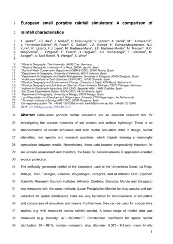
Fig. 4. Measured drop size distributions and calculated Marshall & Palmerdistributions of equal intensities expressed as box plots for total plot (n: 25 on 5positions [WA: n: 3 on one position]). The lower and upper boundaries of eachbox represent the 25th and 75th percentiles, respectively, and the lower and329upper error bars represent the 10th and 90th percentiles, respectively.17

330Fig. 5. Average spatial rainfall distributions for the rainfall simulators (mm h-1; n 3 replicates per simulator).18

331Fig. 6. Average spatial rainfall variability (%) calculated from 3 replicate measurements for each simulator.19

332The rainfall simulator from BA produced the highest intensities at the upper left and right333corners (51-100 mm h-1) and in the middle (45-50 mm h-1). The other collectors on the plot334showed values between 35 mm h-1 and 45 mm h-1. The average deviation from the mean335was highest at the upper left and right corners, with deviations up to 20%.336The intensities for GR were lowest in the first row directly at the outlet (39-60 mm h-1). In337contrast, in most of the other collectors across the plot more than twice the amounts (up to338136 mm h-1) were measured. The average deviation from the mean showed an almost339concentric pattern of rainfall distribution. Central values ranged from 0 to 5% and increased340outwards, with values higher than 20% recorded around the edges.341The rainfall simulator from AL produced a spatial rainfall distribution with intensities below34240 mm h-1 on the front half of the plot. In contrast, the upper half was characterized by high343intensities, most of them

5 124 type of rainfall simulator is the most common device used in semi-arid areas in Europe, 125 especially in Spain, and major differences typically occur in pumps, nozzles and applied 126 intensities. Duration of all simulators is adjustable, only the WA-simulator is limited to three 127 min, due to its compact design. 128 129 Table 1 130 The main characteristics of small scale portable .