Transcription
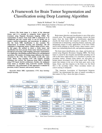
(IJACSA) International Journal of Advanced Computer Science and Applications,Vol. 11, No. 8, 2020A Framework for Brain Tumor Segmentation andClassification using Deep Learning AlgorithmSunita M. Kulkarni1, Dr. G. Sundari2Department of ECE, Sathyabama Institute of Science and TechnologyChennai, IndiaAbstract—The brain tumor is a cluster of the abnormaltissues, and it is essential to categorize brain tumors fortreatment using Magnetic Resonance Imaging (MRI). Thesegmentation of tumors from brain MRI is understood to becomplicated and also crucial tasks. It can be further use insurgery, medical preparation, and assessments. In addition tothis, the brain MRI classification is also essential. Theenhancement of machine learning and technology will aidradiologists in diagnosing tumors without taking invasive steps.In this paper, the method to detect a brain tumor andclassification has been present. Brain tumor detection processesthrough pre-processing, skull stripping, and tumor segmentation.It is employing a thresholding method followed by morphologicaloperations. The number of training image influences the featureextracted by the CNN, then CNN models overfit after someepoch. Hence, deep learning CNN with transfer learningtechniques has evolved. The tumorous brain MRI is classifiedusing CNN based AlexNet architecture. Further, the malignantbrain tumor is classified using GooLeNet transfer learningarchitecture. The performance of this approach is evaluated byprecision, recall, F-measure, and accuracy metrics.Keywords—Brain MRI; segmentation; CNN; deep learning;transfer learningI.INTRODUCTIONBrain tumor detection and classification is one of the activeresearch areas. The segmentation technique extracts the braintumor from the brain MRI, and classification algorithmsclassify the brain tumor into respective categories. It has anessential task in interpreting, extracting features, analyzing, andinterpreting images in many applications. It has been widelyused in brain imaging to classify tissues, detect tumors, assesstumor size, delineating blood cells, and operation preparation.The brain tumor identification, size, shape, and location arecarried using Magnetic Resonance Imaging (MRI). The braintumor is caused by the irregular uncontrolled spreading out ofcells in the brain called trauma. It is classified as primary andsecondary tumors. Primary brain tumors are non-cancer orbenign tumors developed in the brain tumor itself. The braintumor that initiates in the rest of the body parts such as thelungs, breast, and then migrates to the brain over the bloodflow is the secondary tumor. These secondary tumors arecancer-causing or malignant."The American Association of Neurological Surgeons(AANS)" has demonstrated the types of tumors according totheir nature [1]. Fig. 1 shows the types of tumors.Fig. 1. Brain Tumor Classification According to AANS.374 P a g ewww.ijacsa.thesai.org
(IJACSA) International Journal of Advanced Computer Science and Applications,Vol. 11, No. 8, 2020This research aims first to detect the brain tumor from MRI.The tumorous MRIs further classifies using the transferlearning architecture, i.e., AlexNet, into Malignant and benign.The cancerous malignant tumors are also classified into gliomaand meningioma using the GoogLeNet architecture of CNN.The classification architectures are selected based on theiraccuracy by hyper tuning the training parameters. As thedatabase is limited, the transfer learning model helps speed uptraining and improves the job of the classifier.This paper is structured as Section II offers a brief outlineof the recent progress in the brain tumor detection, andclassification aided by Machine Learning (ML) and DeepLearning (DL) algorithms into malignant and benign as well asglioma and meningioma. Section III presents the architectureof the proposed methodology. It includes the brain tumorsegmentation and classification using transfer learning.Quantitative and qualitative analysis is present in Section IV.Section V gives concluded the approach and suggests thefuture direction for this research work.II. LITERATURE SURVEYBrain tumor classification plays a substantial role in thesuggested methodology. In the latest times, the classificationprocess widely uses DL and ML algorithms. This sectionpresents the methods and previous works in brain tumorsegmentation and ML-based classification from MRI.A. Padma et al. [2] introduced segmentation andclassification of the brain tumor in the CT image. It usedDominant Gray Level Run Length Matrix (DGLRLM) as afeature extraction technique. The proposed method for findingtumors in brain CT images with the use of a Support VectorMachine (SVM) classification shows an efficient segmentationalgorithm. Their work aims to combine the DGLRLM andwavelet-based feature extraction techniques. Ideal shapefeatures are selected using a genetic algorithm. SVM usesDGLRLM and wavelet features as input. The average accuracyrate is over 97%.A. Hamamci et al. [3] proposed a brain tumor segmentationapproach for radiotherapy applications. They provide a quickreal-world platform for the classification of tumors with theleast user collaboration to aid researchers along with cliniciansin surgical preparation and assess response to treatment.Importantly, Cellular Automata (CA) focuses on seeded tumorclassification method on MRI, which offered seed selection.First, they build a relationship between CA-based segmentationfor graph-theory techniques to establish that the redundant CAstructure responds to the shortest path problem. The stateconversion performance of the CA followed to estimates theshortest path. Besides, the segmentation problems adjusted thesensitivity factor amplitude for the segmentation problem, anda level set of tumor probability maps generated from CA states.Only adequate clinical data can be collected from the user withclinical practice to reset the algorithm by drawing on thelargest diameter of the tumor.Aneza and Rawat et al. [4] introduced the Fuzzy ClusteringMean (FCM) segmentation approach. The performance of thesegmentation is evaluated based on cluster validationfunctions, processing time, and convergence rate. It achievesan of 0.537% misclassification error using the IntuitionisticFuzzy C-Means (IFCM) method.Ravindra Sonavane et al. [5] present the approach for thesorting of brain MRI classification into malignant and benign.This system used the AdaBoost algorithm. It consists of preprocessing using Anisotropic Diffusion Filtering, featureextraction by Discrete Wavelet Transform (DWT), andclassification by using the Adaboost ML algorithm.Experimental results use 155 MRI images for performanceevaluation.V. Wasule and P. Sonar [6] presented a method for MRIclassification of the brain in malignant versus benign. In thispaper, feature extraction uses the GLCM algorithm. Thissystem uses SVM and K Nearest Neighbors (KNN) for theclassification of malignant vs. benign and low grade vs. highgrade glioma. The clinical dataset is used for malignant andbenign classification, while the BRATS 2012 dataset for highgrade and low-grade glioma classification. The system showsthat SVM performs better.Saleck et al. [7] presented a robust and accurate systemusing the FCM segmentation technique. It extracts thetumorous mass from the MRIs. The presented method aims toavoid problematic estimation by selecting the cluster in theFCM as input data, which can provide us with the data neededto execute mass partitions by fitting only two clusters of pixels.GLCM is used to extract texture properties to obtain theoptimal threshold, which divides between the selected groupand the pixels of other groups, which significantly affects theprecision.M. Rashid et al. [8] examined the MRI image and a methodfor an even clearer vision of the position acquired by the tumor.MRI brain image is an input of the system. This method usedan Anisotropic filter to remove the noise from the brain MRI,SVM used for segmentation followed by a morphologicaloperation.T. Ren et al. [9] proposed the method to solve brain tumorsegmentation. Initially, the irrelevant information is removedfrom the image by histogram equalization. Then, by the studyand research, three segmentation techniques were proposed bythem are FCM, Kernel-based FCM (KFCOM), and WeightedFuzzy Kernel Clustering (WKFCOM). The assessmentdisplays that WKFCOM does better as compared to KFCOM, a2.36% lesser false classification rate.P. Kumar et al. [10] presented a four-step sorting methodfor brain tumor segmentation and classification. The Wienerfilter is used to denoising the image in the initial stage, imagedecomposition in the second stage. Then the combined edgeand texture feature is combined with the Principal ComponentAnalysis (PCA) is performed to minimize the dimension of thefeatures. The last step is the classification step, which classifiesbrain tumors from MRI using SVM classification.S. Kebir et al. [11] provides a supervised approach to detectabnormalities of the brain, predominantly proposing MRIimages in three stages. The first stage is the creation of a DLCNN model, and the next section of tumor segmentation usingthe K-mean clustering. They are introducing CNN models toclassify the abnormality of the MRIs.375 P a g ewww.ijacsa.thesai.org
(IJACSA) International Journal of Advanced Computer Science and Applications,Vol. 11, No. 8, 2020Muhammad Talo et al. [12] suggested the deep transferlearning technique classifies MRI images of the brain asnormal and abnormal. The pre-trained CNN model used theResNet34 algorithm. The database is expands using dataaugmentation techniques. This method is validated on theHarvard Medical School MR dataset [13] and suggests findingadditional abnormalities such as autism, stroke, Parkinson's,and Alzheimer's disease.S. Deepak et al. [14] presented a brain tumor classificationtechnique using GoogLeNet. Brain tumors are classifiedaccording to their nature as glioma, meningioma, and pituitary.Because the classification of brain tumors is comparativelycomplex, the convenience of classification means that there is areasonable degree of deviation in size and shape, which affectsthe classification. This problem is most surprising when itcomes to use traditional ML techniques. To defeat thisproblem, they introduced transfer learning to achieve a higherlevel of learning accuracy compared to the previous model.The significant enhancement was attained even for smallerdatasets. This system suggested GoogLeNet, which is prevalentat the Softmax level, with some modifications for a widevariety of tumor classifications. The CNN focused GoogLeNetmethod attained a better precision of 92.3% that reached 97.8%by using multiclass SVM.III. PROPOSED METHODOLOGYThis section presents brain tumor detection andclassification techniques shown in Fig. 2. The three stages ofthe proposed system are:Fig. 2. Block Diagram of the Brain Tumor Detection and ClassificationSystem.(a)(b)Fig. 3. Brain MRI Samples (a) Tumorous (b) Non-Tumorous.There are many different ways to segment the skull.Among them, skull stripping is the technique that focuses onautomatic segmentation and morphological operation. Fig. 4shows the process of the skull stripping algorithm. Brain Tumor Detection. Benign and Malignant Brain MRI Classification. Glioma and Meningioma Brain MRI Classification.A. Brain Tumor DetectionThe methodology to detect the brain tumor from the brainMRI discusses in this section.1) Tumor Vs. Non-Tumor Dataset: The online data iscollected from the online source for tumorous and nontumorous classification [15]. This dataset consists of 154tumorous MRIs and 91 non-tumorous MRIs. Fig. 3(a) andFig. 3(b). show the sample of tumorous and non-tumorousbrain MRI.2) Pre-processing: In the normalization process, theintensity falls within the range of pixel values converted into[0 1] range. In this process, each pixel intensity is divided bythe maximum intensity values within an image. Normalizationcan create binary thresholding by creating a more extensivesource. Such MRI images can help to prevent classificationsaffected by variations of grayscale value.3) Skull stripping: Skull stripping is a necessaryprocedure in the biomedical image examination for theefficient analysis of brain tumors from brain MRI [16]. Iteliminates the non-brain parts like skin, fat, and skull from thebrain MRI.Fig. 4. The flow of the Skull Stripping Process.376 P a g ewww.ijacsa.thesai.org
(IJACSA) International Journal of Advanced Computer Science and Applications,Vol. 11, No. 8, 20204) Brain tumor detection and area calculation: Thefollowing methods achieve the brain tumor segmentation fromthe brain MRIs: Initially, the input brain MRIs are preprocessed and converted into a binary image by thresholdingtechnique and morphological operation. The thresholdingprocess chooses 128 as a threshold value. The pixel whosevalues are more significant than the defined threshold issubject to 1, while rest are subject to 0. It makes two areasbuilt around the tumor region. The conversion of a grayscaleimage into a binary image is done by (1).1𝑓𝑔(𝑥,𝑦) 0𝐼(𝑥, 𝑦) 𝑇𝑒𝑙𝑠𝑒(1)Where I(x, y) is the intensity value of the grayscale pixeland fg(x,y) is the resultant binary pixel.In the next step, morphological processing is performed byerosion and dilation process on binary image to gain the properboundary of the tum while dilation operation filling the gapswithin the detected object using Erosion operation. Themorphological process uses a small mask (3x3 or 5x5) ofdifferent sizes, and it is applied over the image known as thestructuring element. This element has various shapes, such aslines, disk, diamonds, etc.The erosion of an image is given by𝐴 𝐵 {𝑧 𝐸 𝐵 𝐴}(2)𝐴 𝐵 𝑏 𝐵 𝐴𝑏(3)𝐴𝑟𝑒𝑎 𝑛𝑖 0 𝑖 1(4)The dilation of an image is given byAfter the detection of tumors, calculates the area of thetumor for further processing (Eq. (4)).B. Benign and Malignant brain MRI ClassificationOnce the tumor is detected, the brain MRI is analyzing forthe malignancy of the image. In this section, the CNN basedAlexNet transfer learning architecture is utilized for trainingand classifying the brain MRI for classification.1) Benign Vs. Malignant Dataset: The classification ofbrain tumors into benign and malignant uses clinical datasetcollected from the hospital. The database comprises of benignand malignant MRI images [17]. The complete databasedistribution is tabulated in Table I. The database has MRIsthat are pre-processed by brain augmentation andsegmentation methods after separating testing and trainingdata. Finally, it presents the performance of the training andtesting process.comparatively lesser, then that DL model may begin toremember the features that are too explicit to that particulardatabase, which leads to overfitting. Thus to avoid theoverfitting dilemma, the dataset should be huge withsignificant dissimilarity, but this is an extremely puzzling taskin this scenario of clinical images. One remedy could be toaugment the existing database synthetically. Such a practice isgeneral when dealing with image-based data [18]. Dataaugmentation includes various methods like flipping, rotation,adding noise, scaling translation, resizing, perspectivetransform, etc. The parameters related to data augmentationused in the proposed method are as charted in Table II.3) Training using AlexNet: In the presented work, the pretrained CNN network, referred to as 'AlexNet,' is employed.AlexNet is among the renowned architecture that comprises ofConvolution Layers (CL) (five in number), max-poolinglayers (three in number), and Fully Connected Layer (FCL)(three in number). It was training for classifying 1000different objects [20]. There may be few objects that don't gowith the original dataset. So the network can have specificlayers kept back to identify those non-belonging objects.Fig. 5. illustrates the architecture of AlexNet.With the actual size of the dataset, training a DL modelfrom zero is inadequate since there is a tremendous rise in thenumber of training images. Pre-trained AlexNet architectureemploys three different steps to avoid this situation. In the firststep, the classification layer of the AlexNet replaces with thesoftmax layer that includes two categories (benign andmalignant). Then in the second step, the weights are modifiedand backpropagate to retrain the images. The learning rate isset to a lesser value so that the weights of the CL do not alterintensely. At the same time, the weights of the FLC setasystematically. The stochastic gradient descent algorithm isemployed to appraise the weight depending on the inputdatabase of brain MRI. This procedure helps in achieving theoptimum weights of the exact network system.TABLE I.DATABASE DISTRIBUTION FOR MALIGNANT VS. BENIGNCLASSIFICATIONType of TumorTrainingTestingBenign MRI7525100Malignant MRI7525100TABLE II.Total ImageDATA AUGMENTATION PARAMETERS FOR ALEXNETSr. NoParameterValue1Random X Reflection12Random Y Reflection0MRIs of the dataset are pre-processed and remove nonbrain parts by skull stripping, as illustrated in Sections III(A(2)) and III (A(3)) of this paper.3Random Rotation[0,0]4Random X Scale[1,1]5Random Y Scale[1,1]2) Data augmentation: DL architecture requires anenormous amount of data that includes variation. In transferlearning, data augmentation forms happen to be a vitalcomponent of the pre-processing. If the database is6Random X Shear[0,0]7Random Y Shear[0 0]8Random X Translation[-10 10]9Random Y Translation[-10 10]377 P a g ewww.ijacsa.thesai.org
(IJACSA) International Journal of Advanced Computer Science and Applications,Vol. 11, No. 8, 2020TABLE IV.Fig. 5. Architecture of AlexNet.C. Glioma and Meningioma brain MRI ClassificationThis section presents the GoogLeNet algorithm for theclassification of brain MRI into Glioma and Meningioma.DATA AUGMENTATION PARAMETERS FOR GOOGLENETSr. NoParameterValue1Random X Reflection12Random Y Reflection03Random Rotation[0,0]4Random X Scale[1,1]5Random Y Scale[1,1]6Random X Shear[0,0]7Random Y Shear[0 0]8Random X Translation[-10 10]9Random Y Translation[-10 10]1) Glioma Vs Meningioma Dataset: This approach uses aclinical dataset of Glioma and Meningioma brain MR imagesas an input. The dataset is collected from the Cancer Hospitaland validated by the radiologist. The database distribution fortraining and testing is as shown in Table III.The skull stripping is the initial step used to remove thenon-brain part and select the region of interest. The process ofskull stripping is shown in Sections 3.1.2 and 3.1.3 of thispaper.2) Data augmentation: Data augmentation includesvarious methods such as flipping, rotation, adding noise,scaling translation, resizing, perspective transform, etc. Theparameters related to data augmentation of the proposedmethod are as charted in Table IV.3) Training using GoogLeNet: VGG-16 has CL piled oneabove the other while GoogLeNet has pooling and CL in aparallel fashion, which helps in the feature extraction throughvarious kernel sizes. It enhances the network depth and ahigher performance level. Also, the network employs 1 1convolution to govern the volume size passed for additionalprocessing in the inception module. It is nothing but acollection of pooling and convolution operations executedparallelly to extract features with the aid of various scales.GoogLeNet network consists of 24 million parameters due towhich it has lesser computing complexities as associated withVGG-16 and AlexNet. Instead, of FCL network employs aGlobal Average Pooling layer. Eventually, in ILSVRC-2014,GoogLeNet had got an error of 6.67%. The GoogLeNetarchitecture is as displayed in Fig. 6.TABLE III.DATABASE DISTRIBUTION FOR GLIOMA VS. MENINGIOMACLASSIFICATIONType of TumorTotal ImageTrainingTestingGlioma MRI27121853Meningioma MRI987919Fig. 6. Layer Architecture of GooLeNet.378 P a g ewww.ijacsa.thesai.org
(IJACSA) International Journal of Advanced Computer Science and Applications,Vol. 11, No. 8, 2020IV. RESULT AND DISCUSSIONThis section presents the Qualitative and Quantitativeanalysis of the proposed system. This system uses 64-bitMATLAB 2019a software. This system uses a single CentralProcessing Unit (CPU) to train the network. The quantitativeanalysis evaluates precision, recall, F-measure and accuracyevaluation metrics, and mathematically denoted as:Precision Recall TPTPTP FNF measure 2 XAccuracy (5)TP FPTable V shows the input brain MRI in the second column.Images in the first three rows contain non-tumorous images,while the next three rows contain tumorous images. Therespective segmented output is shown in the third column. Thenon-tumorous images contain no white pixels (1's); hence %area of the tumor is zero while the tumorous images showrespective values. The area of the tumor could help the doctorsin the analysis and planning of surgery.TABLE V.(6)Sr. NoPrecisionXRecall(7)Precision RecallTP TNANALYSIS OF BRAIN TUMOR SEGMENTATION AND % AREA OFTHE TUMORInput ImageSegmented tumor% area ofthe tumor(8)TP TN FP FNTrue Positive (TP) is referring to as a benign identifies asa benign (or glioma is identifying as glioma).True Negative(TN) is referring to as a malignant identified asa malignant (or meningioma is identifying as meningioma).False Positive(FP) is referring to as a benign identified as amalignant (or glioma is identifying as meningioma).False Negative(FN) is referring to as a malignant identified asa benign (or meningioma identifying as glioma).10203041.6656.803963.0685A. Analysis of Brain Tumor Detection methodThe results of the tumor detection from brain MRI is asshown in Fig. 7(a-f).The input brain MRI image is as shown in Fig. 7(a), ischosen for analysis. First, the image is pre-processed using amedian filter and then binarized using the thresholding method.The binary mask is again processed by erosion and dilationoperations and selects the most massive mask, as displayed inFig. 7(b). This mask is multiplied with the input image to get askull stripped image, as shown in Fig.7(c). The brain tumorsegmentation uses the thresholding method to select a region ofinterest. Threshold output, as displayed in Fig. 7(d). Thedetected tumor is shown in Fig. 7(e) and declared as atumorous image with the percentage of area covered by thetumor in the brain MRI Fig. 7(f).(a)(b)(c)(d)(e)(f)Fig. 7. Tumor Detection: (a) Input Image (b) Binary Mask Skull (c)Stripped Image (d) Segmented Tumor (e) Detected Tumor (f) Output Image(Shows Tumorous and % of the Area).379 P a g ewww.ijacsa.thesai.org
(IJACSA) International Journal of Advanced Computer Science and Applications,Vol. 11, No. 8, 2020B. Analysis of Benign and Malignant Classification MethodThe qualitative analysis of malignant and benignclassification using the AlexNet CNN algorithm is as displayedin Fig. 8.Qualitative analysis of benign vs. malignant classificationis performed on the testing database. The input samples of thebenign and malignant brain MRI areas are shown in Fig. 8(a)and Fig. 8(c) and a resultant class of the AlexNet are displayingin Fig. 8(b) and Fig. 8(d), respectively.The training progress of AlexNet is as displayed in Fig. 9.The quantitative analysis of malignant and benignclassification using the AlexNet, Vgg16, ResNet18, ResNet50,and GoogLeNet CNN algorithm is as displayed in Table VI,and its graphical analysis is showing in Fig. 10.TABLE VI.COMPARATIVE ANALYSIS OF BENIGN AND MALIGNANTCLASSIFICATION METHODSMethodsPrecisionRecallF-measureSVM [6]10.760.8636KNN [6]0.880.730.7999Proposed Method (AlexNet)0.937510.9677419Proposed Method (Vgg16)0.550.50.5238095Proposed Method (ResNet18)0.90.7830.8372093Proposed Method (ResNet50)0.250.8330.3846154Proposed Method (GoogLeNet)0.810.8888889This approach is more generalized and shows betteraccuracy on the testing dataset. The relative examination of thissystem with state-of-art methods shows the dominancy of theproposed AlexNet method.Fig. 10. Performance Analysis of Proposed Systems with State of the ArtMethod for Malignant and benign Classification.(a)(b)(c)(d)C. Analysis of Glioma and Meningioma ClassificationMethodQualitative analysis performs on the testing dataset forclassification of Glioma vs. Meningioma. The results aredisplaying in Fig. 11. The input samples of the Glioma andMeningioma brain MRI display in Fig. 11(a), and Fig. 11(c)and a resultant class of the GoogLeNet are shown in Fig. 11(b)and Fig. 11(d), respectively.Fig. 8. Qualitative Analysis of the benign and Malignant Classificationusing AlexNet (a) (c) Input MRI Image (b) (d) Output Classified Image.Fig. 9. Training Progress of AlexNet Transfer Learning Architecture forbenign and Malignant Brain MRI.(a)(b)(c)(d)Fig. 11. Qualitative Analysis of the Glioma and Meningioma Classificationusing AlexNet (a) (c) Input MRI Image (b) (d) Output Classified Image.380 P a g ewww.ijacsa.thesai.org
(IJACSA) International Journal of Advanced Computer Science and Applications,Vol. 11, No. 8, 2020The approach of GoogLeNet is more generalized andshows better accuracy on the testing dataset. The relativeanalysis of the proposed system with state-of-art approachesshows the dominancy of the proposed GoogLeNet approach.V. CONCLUSIONFig. 12. Training Progress of GoogLeNet Transfer Learning Architecture forGlioma and Meningioma Brain MRI.The training progress of GoogLeNet is as displayed in Fig.12.The quantitative analysis of malignant and benignclassification using the AlexNet, GoogLeNet, ResNet18, andResNet50 CNN algorithm is as displayed in Table VII.The graphical analysis of the proposed approaches withstate of the art method is given in Fig. 13.TABLE VII.COMPARATIVE ANALYSIS OF GLIOMA AND MENINGIOMACLASSIFICATION METHODSMethodsPrecisionRecallF-measureAccuracySVM and KNN [19]---0.88Proposed Method(AlexNet)0.88630.9750.92850.9047Proposed Method(Vgg16)0.65910.85290.89660.6667Proposed Method(ResNet18)0.93180.87230.90100.85Proposed Method(ResNet50)0.88630.90690.89650.85Proposed Method(GoogLeNet)0.9510.97430.9750In this paper, a technique for brain tumor detection andgrading of tumorous MRIs into malignant and benign as wellas malignant brain MRI into glioma and meningioma isproposed. The brain tumor detection is executed by preprocessing techniques followed by skull stripping and braintumor segmentation. This approach promisingly segments thebrain tumor from MRI. The tumorous images are furtherclassified into malignant and benign using CNN based AlexNettransfer learning algorithms. The proposed method achieved aprecision of 0.9375, recall of 1, and f-measure of 0.9677.Similarly, the malignant MRI further classified into Gliomaand Meningioma using CNN based GoogLeNet transferlearning algorithm. GoogLeNet model successfully got aprecision of 0.95, recall of 1, f-measure of 0.9743, andaccuracy of 0.9750. The proposed approaches (malignant vs.benign or glioma vs. meningioma) shows better results thanexisting methods.The deep neural networks, particularly CNN, are rarelyused for boundary detection problems. Therefore, the uses ofdeep neural networks can be a future direction for brain tumorsegmentation and detection problem. In addition to this, the3D brain boundary detection can be possible with this method.In the case of classification of dissimilar types of brain MRI(malignant vs. benign or glioma vs. meningioma), the systemcan be made more robust and generalized by training the deepneural networks on extensive data. Also, the system will beextended for further classification of low-grade and high-gradeglioma as well as meningioma.[1][2][3][4][5][6][7]Fig. 13. Performance Analysis of Proposed Systems with State of the ArtMethod.REFERENCESClassification of Brain Tumors: rain-Tumors. Access on 29 June 2020.A PADMA and R.Sukanesh, "Automatic Classification andSegmentation of Brain Tumor in CT Images using Optimal DominantGray level Run length Texture Features" International Journal ofAdvanced Computer Science and Applications(IJACSA), 2(10), pp. 5359, 2011.A. Hamamci, N. Kucuk, K. Karaman, K. Engin, and G. Unal, "TumorCut: Segmentation of Brain Tumors on Contrast Enhanced MR Imagesfor Radiosurgery Applications," in IEEE Transactions on MedicalImaging, vol. 31, no. 3, pp. 790-804, March 2012.Aneja, Deepali, and Tarun Kumar Rawat. "Fuzzy Clustering Algorithmsfor Effective Medical Image Segmentation." International Journal ofIntelligent Systems and Applications, Vol. 5, pp. 55-61, 2013.R. Sonavane and P. Sonar, "Classification and segmentation of braintumor using Adaboost classifier," 2016 International Conference onGlobal Trends in Signal Processing, Information Computing andCommunication (ICGTSPICC), Jalgaon, pp. 396-403, 2016.V. Wasule and P. Sonar, "Classification of brain MRI using SVM andKNN classifier," 2017 Third International Conference on Sensing,Signal Processing and Security (ICSSS), Chennai, pp. 218-223, 2017.M. M. Saleck, A. ElMoutaouakkil, and M. Mouçouf, "Tumor Detectionin Mammography Images Using Fuzzy C-means and GLCM TextureFeatures," 2017 14th International Conference on Computer Graphics,Imaging and Visualization, Marrakesh, pp. 122-125, 2017.381 P a g ewww.ijacsa.thesai.org
(IJACSA) International Journal of Advanced Computer Science and Applications,Vol. 11, No. 8, 2020[8][9][10][11][12][13][14]M. H. O. Rashid, M. A. Mamun, M. A. Hossain, and M. P. Uddin,"Brain Tumor Detection Using Anisotropic Filtering, SVM Classifierand Morphological Operation from MR Images," 2018 InternationalConference on Computer, Communication, Chemical, Material andElectronic Engineering (IC4ME2), Rajshahi, pp. 1-4, 2018.Ren, T., Wang, H., Feng, H., Xu, C., Liu, G., & Ding, P, "Study on theimproved fuzzy clustering algorithm and its application in brain imagesegmentation," Appl. Soft Comput., Vol. 81, pp. 1-9, 2019.Preetham Kumar and Vijayakumar B, "Brain Tumour MR ImageSegmentation and Classification Using by PCA and RBF Kernel BasedSupport Vector Machin
Classification using Deep Learning Algorithm . Sunita M. Kulkarni. 1, Dr. G. Sundari. 2. Department of ECE, Sathyabama Institute of Science and Technology . Chennai, India . Abstract—The brain tumor is a cluster of the abnormal tissues, and it is essential to categorize brain tumors for treatment using Magnetic Resonance Imaging (MRI).