Transcription
Building ARIMA and ARIMAX Models forPredicting Long-Term Disability Benefit ApplicationRates in the Public/Private SectorsSponsored bySociety of ActuariesHealth SectionPrepared byBruce H. AndrewsMatthew D. DeanRobert SwainCaroline ColeUniversity of Southern MaineAugust 2013 2013 Society of Actuaries, All Rights ReservedThe opinions expressed and conclusions reached by the authors are their own and do not represent any official position or opinionof the Society of Actuaries or its members. The Society of Actuaries makes no representation or warranty to the accuracy of theinformation.
EXECUTIVE SUMMARYUsing the Social Security Disability Insurance benefit claim rate as a proxy, this studyinvestigates two statistical approaches to forecasting long-term disability benefit claims. Theresults are extendable and should prove useful for insurance carriers who wish to predict shortterm future levels of long-term disability benefit claims. The study demonstrates that both theautoregressive integrated moving average (ARIMA) and autoregressive integrated movingaverage with exogenous variables (ARIMAX) methodologies have the ability to produceaccurate four-quarter forecasts.First built was an ARIMA model, which produces forecasts based upon prior values in the timeseries (AR terms) and the errors made by previous predictions (MA terms). This typically allowsthe model to rapidly adjust for sudden changes in trend, resulting in more accurate forecasts.Next built was an ARIMAX model, which is very similar to an ARIMA model, except that italso includes relevant independent variables. While the inclusion of exogenous variables addscomplexity to the model-building process, the model can capture the influence of external factors(e.g., the state of the economy) as well as management controllables (e.g., elimination periodduration).The superior performance of both the ARIMA and ARIMAX models against the commonly usedseasonally adjusted four-quarter moving average (SAMA) model can be seen in the followinggraph. Both models’ cumulative errors tend to remain close to zero, while the SAMA model’scumulative errors deviate from zero more dramatically. The additional beneficial impact of 2013 Society of Actuaries, All Rights ReservedUniversity of Southern Maine
including exogenous variables in the model can also be seen by the ARIMAX model’scumulative errors remaining closer to zero.Cumulative Errors Resulting from 25 4-QuarterHoldout-Forecasts (Q1 1988–Q4 2012)SAMAARIMAARIMAX98Cumulative Forecast 32011Q22012Q12012Q4-2QuarterThe benefits to an insurance carrier who is able to accurately predict the disability benefit claimsrate are clear. The carrier will be in a much better position to make a wide range of criticalplanning decisions that are affected by the claims rate, including establishing appropriate reservelevels to service approved claims. This study utilized two powerful techniques to forecast SSDIapplication rates for benefit claims. Social Security data were chosen primarily because theywere readily publically available and familiar to many insurance analysts. However, the modelbuilding exercise detailed in the report can be readily applied to private-sector long-termdisability benefit claim application rates. 2013 Society of Actuaries, All Rights ReservedUniversity of Southern Maine
BUILDING ARIMA and ARIMAX MODELSforPREDICTING LONG-TERM DISABILITY BENEFIT APPLICATION RATESin thePUBLIC/PRIVATE SECTORS 2013 Society of Actuaries, All Rights ReservedUniversity of Southern MainePage 1
ACKNOWLEDGEMENTSThe authors are extremely grateful for the financial support provided by the Society ofActuaries and for their compassion in granting “no cost” extensions. In addition, the authors alsowish to thank the Maine Center for Business and Economic Research for its generous financialsupport. 2013 Society of Actuaries, All Rights ReservedUniversity of Southern MainePage 2
1. INTRODUCTION1.1 Purpose of the StudyThe Maine Center for Business and Economic Research (MCBER) at the University of SouthernMaine, in partnership with the Society of Actuaries (SOA), conducted a predictive modelbuilding exercise to statistically examine and incorporate factors that influence long-termdisability (LTD) application rates. This report documents that study. Social SecurityAdministration (SSA) claims-experience data were selected for the model building because theyare publicly available and representative (in varying degrees) of the private-sector LTD claimsexperience. Private LTD carrier data were deemed inappropriate for use in this study becausethey vary in form, level of detail and their period of collection. Further, it was thought that LTDcarriers would find it awkward to share or pool their data with other carriers because theyfrequently compete in the same markets.Many of the phenomena that drive Social Security disability application rates are likely toinfluence LTD application rates for private carriers, which means that exogenous variables thatare significant predictors of Social Security Disability Insurance (SSDI) application rates arelikely to be strong predictors for private carriers as well. Also, the future experience of at leastsome private-sector carriers was expected to display a statistical relationship with the applicationrates projected for Social Security disability.This study focuses most heavily on the autoregressive integrated moving average withexogenous variables (ARIMAX) methodology, which has the capacity to identify the underlyingpatterns in time-series data and to quantify the impact of environmental influences. This provides 2013 Society of Actuaries, All Rights ReservedUniversity of Southern MainePage 3
the ARIMAX modeler with the capacity to isolate the influences of high-impact changes of bothan external nature (e.g., competitors’ activities, the economy and governmental regulations) andan internal nature (e.g., policy coverage, product pricing and target markets). It is also importantto note that ARIMAX model building can be reduced/simplified to pure autoregressiveintegrated moving average (ARIMA) model building if the forecaster/modeler wishes to examinehistorical behavior and make projections employing only statistically identified historicalpatterns/relationships.The target audience for this report is the actuary who either has a basic working knowledge ofapplied multiple-linear-regression model building or is willing to invest the energy toacquire/recover it. This prerequisite level of understanding of multiple-regression analysis is thatwhich is typically derived from the one or two 3-credit (noncalculus-based) undergraduatecourses in applied business statistics required at nationally accredited business schools. Asfurther encouragement for the tentative reader to press forward, the two student co-authors ofthis report, Bob Swain and Caroline Cole, have completed only the six credits of undergraduatelevel statistics required by the business school at the University of Southern Maine.1.2 BackgroundTo coarsely evaluate the strength of the potential relationship between the application rates forSSDI and those of group LTD carriers, annual data from 2004–10 from 12 of the largest privatesector carriers were examined. Six of the 12 carriers had annual application rates that weresignificantly correlated ( 0.10) with SSDI’s annual application rates at lags of 0, 1 and/or 2.Four of these six exhibited one or more significant positive correlations; the other two displayed 2013 Society of Actuaries, All Rights ReservedUniversity of Southern MainePage 4
significant negative correlations, one at lag 1 and the other at lags 1 and 2. (It is important to notethat the coarseness of the data and the small sample [n 7] placed serious constraints on thisstatistical analysis.)Accurate prediction of future application rates for long-term disability benefits is a majorconcern for private insurance carriers as well as the Social Security Administration. In both theprivate and public sectors, the number of claims filed is a key input to many planning decisions.For example, in both sectors, the proper level of reserves required to service approved claimsneeds to be established, mechanisms to generate revenue streams must be created to maintainappropriate reserve levels, and claims processing and management capacity requirements mustbe estimated. Unfortunately, application rates are extremely volatile because they are largelydriven by forces external to the insurer, be it the SSA in the public sector or an LTD provider inthe private sector. For example, at the national level, SSDI applications increased substantially1during six of the seven U.S. recessions between 1965 and 2012.2 Further, a December 2011article in the Wall Street Journal,3 titled “Jobless Tap Disability Fund,” reported on the findingsof researchers who have studied the interaction between the condition of the U.S. economy andthe SSDI application rate. Some of their findings are summarized below. Professor Mark Duggan at the University of Pennsylvania studied the relationshipbetween the U.S. unemployment rate and the application rate for SSDI benefits, and“estimates that the higher unemployment rate [in 2011 compared to 2007] accountsfor 3,000 additional people applying for benefits each week.”1Social Security Administration, “Disabled Workers.”Wikipedia contributors, “List of recessions in the United States.”3Paletta and Searcey, “Jobless Tap Disability Fund.”2 2013 Society of Actuaries, All Rights ReservedUniversity of Southern MainePage 5
Steven Goss, chief actuary of the Social Security Administration, “told Congress that the 2008–09 recession led to a higher rate of ‘disability incidence’ than any otherperiod except for the economic downturn in 1975.” Professor Matthew Rutledge at Boston College studied the relationship between timeleft until unemployment benefits expire and the likelihood an individual would applyfor SSDI benefits, and found that the unemployed are “significantly more likely toapply when [unemployment payments are] ultimately exhausted,” indicating thatlong-term unemployment is positively linked to the SSDI application rate. Massachusetts Institute of Technology professor of economics David Autor summedup his sentiments this way: “To a very large extent, [SSDI] is our big welfareprogram.”Some of the other 16 major determinants of the disability application rate listed in ActuarialStudy No. 118 produced by the SSA’s Office of the Actuary4 include the strength of regionaleconomies, demographic shifts, levels of employment/unemployment and levels of inflation.1.3 The ARIMAX MethodologyProper ARIMAX model building has six statistical assumptions that must be addressed and readdressed as iterative model building progresses. These six assumptions also provide theunderpinnings for rigorously performed multiple-regression analysis. While the rules of properlyperformed regression analysis are rarely fully honored by nonacademic practitioners, whensatisfied, they normally lead to much-improved model-building results.4Zayatz, “Social Security Disability.” 2013 Society of Actuaries, All Rights ReservedUniversity of Southern MainePage 6
Simply put, an ARIMAX model can be viewed as a multiple regression model with one or moreautoregressive (AR) terms and/or one or more moving average (MA) terms. Autoregressiveterms for a dependent variable are merely lagged values of that dependent variable that have astatistically significant relationship with its most recent value. Moving average terms are nothingmore than residuals (i.e., lagged errors) resulting from previously made estimates.So, for example, a nameless time-series dependent variablemight be well estimated by aproperly weighted combination of the following four right-hand-side (RHS) variables.1. the value of the independent variableat time2. the immediately preceding value of the dependent variableat time3. the immediately preceding value of the dependent variableat time4. the estimation error produced by the model at timeThis single-independent-variable, multiple-regression-like model for estimating the dependentvariablerelies on the predictive value of the independent variable(unlagged), the dependentvariable itself (lagged by 1), the dependent variable again (lagged by 2) and a previouslyproduced error term (lagged by 4). That is,,where,,andare estimated coefficients.As implied by its shortened acronym, the pure ARIMA model-building methodology employsonly lagged values of the dependent variable (i.e., AR terms) and lagged values of errorspreviously produced by the model (i.e., MA terms). The I in ARIMA refers to integrated andindicates that the dependent variable time series has been differenced one or more times to make 2013 Society of Actuaries, All Rights ReservedUniversity of Southern MainePage 7
the time series stationary before model building begins. (Note: Practically speaking, stationarityimplies that the mean and the variance of the time series are not changing over time.) So, forexample, the quarterly application rate for SSDI benefits time series used illustratively in thisreport has displayed a strong overall pattern characterized by both an upward trend and quiteregular quarterly seasonality. As discussed in Section 2.1, to remove the quarterly seasonality,the raw data were differenced by four and then differenced by one to remove the upward trend.The core difference between formal ARIMAX modeling and the more commonly used multipleregression modeling is that the ARIMAX modeling rigorously adheres to all six of the statisticalassumptions underlying regression modeling. Section 2.2 explains these six assumptions. TheARIMAX model-building algorithm flowchart (Figure 8) makes clear the complexity of theiterative process. This level of complexity sometimes discourages model builders from fullyadhering to the full set of six key assumptions required for proper regression modeling.Assumption 3 provides one example of the complexities of meticulously executed regressivemodeling in that proper interpretation of the significance levels ( -values) of regression-modelcoefficients requires that the residuals produced by the model under scrutiny are normallydistributed with a mean of zero, a constant variance and (most importantly) with no serialcorrelation. To satisfy these formal assumptions, it is frequently necessary to model the residualswith ARIMA tools, which often forces originally identified, logically attractive independentvariables to lose their significance and to leave the model. This removal of independent variablesthat appeared to be strong candidates changes the form and character of the residuals and mayresult in a complete restart of the model-building process. 2013 Society of Actuaries, All Rights ReservedUniversity of Southern MainePage 8
To address the complex, iterative nature of the ARIMAX model-building process when the poolof explanatory-variable candidates is large, MCBER built a system of integrated SAS5 softwareroutines to automate the search for the optimal or near-optimal combination of exogenousvariables, and AR and MA terms. The resulting ARIMAX models are statistically correct in allregards. Additionally, the composition of both models built using the SAS routines on theillustrative quarterly SSDI-application-rate data set (Q1 1982–Q4 2012) are very intuitivelyappealing. After differencing by four (to remove seasonality) and then one (to remove trend), the(AR1, AR3, AR10, MA4) ARIMA model produced the best fit with a mean error of 0.005901and a standard error of 0.0138 for the residuals. The -values for the coefficients for the AR1,AR3, AR10 and MA4 terms were 0.0002, 0.0035, 0.0045 and 0.0001, respectively. For thedoubly differenced time series, this means that the ARIMA model was built by weighting themost recent actual, the actual three quarters earlier, the actual 10 quarters earlier and theestimation error made four quarters earlier. That is,.The best-fitting ARIMAX model (not coincidentally) has a structure similar to the previousARIMAX model for the “nameless” dependent variable introduced on Page 7. The AR1 and MA4terms from the ARIMA model were accompanied by wage-and-salary employment (wse) (lag 0) andan AR2 term. That is,.5http://www.sas.com 2013 Society of Actuaries, All Rights ReservedUniversity of Southern MainePage 9
This model produced a mean error of 0.004823 and a standard error of 0.0130. The -value forthe coefficients of the AR1, MA4 and the independent variablewere all 0.0001, and the -values for the AR2 term was 0.0058. The fitting and forecasting capacities of the ARIMA andARIMAX models are discussed in further detail on pages 50-52.1.4 Comparison of ARIMAX and SAMA ModelsTo examine the relative precision of the best-fitting ARIMAX model, its fit performance wascompared against that of the commonly used seasonally adjusted four-quarter moving average(SAMA) model. Figure 1 shows the 20 most recent actual quarterly SSDI application rates andthe fit estimates produced by each model. The ARIMAX model clearly does a better job ofestimating the actual application rates, particularly during periods of steady rising or declining. 2013 Society of Actuaries, All Rights ReservedUniversity of Southern MainePage 10
Figure 1. A comparison of the ARIMAX and SAMA models’ fit estimates with the actualdata.ActualsARIMAXSAMA5.5Application Rate / 1000 Insured5.2554.754.54.2543.75QuarterThe absolute values of the estimation errors of the two models are compared in Figure 2, whichfurther demonstrates the ARIMAX model’s superior precision. 2013 Society of Actuaries, All Rights ReservedUniversity of Southern MainePage 08Q42008Q32008Q22008Q13.5
Figure 2. A comparison of the ARIMAX and SAMA models’ absolute errors.ARIMAXSAMA0.800000.70000Absolute 2008Q32008Q22008Q10.00000QuarterThe mean absolute percent errors (MAPEs) and mean absolute deviations (MADs) for bothmodels over all 116 quarters for which both models produce estimates (Q1 1984–Q4 2012) andfor the most recent 20 quarters (Q1 2008–Q4 2012) are shown in Chart 1.Chart 1. A comparison of the ARIMAX and SAMA models’ goodness-of-fit over twodifferent time horizons.Q1 1984–Q4 2012MAPEMADQ1 2008–Q4 54%0.21 2013 Society of Actuaries, All Rights ReservedUniversity of Southern MainePage 12
Once again, the ARIMAX model clearly outperforms the SAMA model based on its lowerMAPEs and MADs for both time periods. In comparison with the SAMA model, the ARIMAXmodel’s MAPEs improve by 24 percent and 37 percent, and its MADs improve by 29 percentand 38 percent.1.5 The Dependent VariableWhile disability insurance award rates (i.e., approval rates) are somewhat influenced by thepreviously mentioned 16 factors, they are also determined by forces internal to the insuranceprovider such as organizational goals, strategies, policies and practices created and administeredfrom within. This tends to reduce the volatility in approval rates and makes them morepredictable than application rates. Not surprisingly, as seen in Figure 3, the application rates forSSDI among insured workers have exhibited much more variability than the acceptance ratesamong SSDI applicants. During the 31-year period of this study (1982–2012), the quarterlyapplication rate per 1,000 insured workers ranged from a low of 1.929 in Q4 1999 to a high of5.292 in Q1 2011, a rise of almost 274 percent. Over the 124 quarters in the data set, theapplication rate mean was 3.046 and the standard deviation was 0.869, yielding a coefficient ofvariation () of 0.285. During the same period, the quarterly award rate, which is theproportion of applications approved, was relatively flat, ranging from 0.255 to 0.558, with amean of 0.411 and a standard deviation of 0.063, yielding a considerably smaller coefficient ofvariation of 0.153. (Note that the coefficient of variation for application rates is 86.3 percentlarger than that for award rates.) Figure 3 makes clear the contrast in the long-term slope and thevolatility of the two time series. 2013 Society of Actuaries, All Rights ReservedUniversity of Southern MainePage 13
Figure 3. Application and award rates for social security disability benefits.Award Rate / ApplicationApplication Rate / 1000 1Q22012Q12012Q40QuarterThis study focuses on modeling the more highly volatile, publicly available quarterly SSDIapplication-rate/1000 insured time series presented in Figure 3. It serves well as a surrogate forprivate-sector submitted LTD claims experience in building time-series forecasting models.While the application-rate time-series patterns in the private sector are not created by all of thesame forces that drive public-sector demand for disability payments, there are certainly manyoverlaps. In both settings, regional and national economic conditions heavily influence the rateof applications as do medical advancements and breakthroughs in the treatment of specificdisorders. Other common influences include demographic shifts (e.g., aging baby boomers),technological improvements that can enhance one’s ability to work and level of participation offemales in the workforce. 2013 Society of Actuaries, All Rights ReservedUniversity of Southern MainePage 14
2. CONSTRUCTION AND VALIDATION OF ARIMA AND ARIMAX MODELSSection 2.1, Construction and Validation of an ARIMA Model, focuses on explaining andillustrating the steps in the methodology for constructing a pure ARIMA model. This illustrationemploys the previously introduced 124-point quarterly SSDI-application-rate time series (Q11982–Q4 2012). This discussion also includes all of the statistical assumptions that must besatisfied for an ARIMA model to be valid. Results from the analysis of residuals from finalARIMA and ARIMAX models are examined to ensure they meet the necessary conditions.Model-fitting results are then presented and evaluated using standard goodness-of-fit measuresproduced by the fitting process. In addition, the accuracy/precision of the holdout forecastsproduced by the final pure ARIMA model are examined.Section 2.2, Construction and Validation of an ARIMAX Model, is heavily patterned afterSection 2.1, but focuses on explaining and illustrating the step-by-step methodology for buildingand validating an ARIMAX model. This discussion also includes an explanation of the muchexpanded series of statistical assumptions that must be satisfied for an ARIMAX model to bevalid. In keeping with the ARIMA discussion in Section 2.1, results from the analysis ofresiduals are reviewed and the quality of the ARIMAX model is evaluated in the context of bothin-sample fitting and holdout-sample forecasting. Lastly, both sets of goodness-of-fit statisticsare compared with their counterparts produced by the pure ARIMA model to assess theincremental explanatory value contributed by the exogenous variables. 2013 Society of Actuaries, All Rights ReservedUniversity of Southern MainePage 15
2.1 Construction and Validation of an ARIMA ModelThe AR (autoregressive) in ARIMA refers to previous (i.e., lagged) values of the dependentvariable time series. MA (moving average) refers to lagged error terms (i.e., residuals) created bythe ARIMA model’s inability to produce perfectly accurate estimates. So, ARMA (ARIMAwithout I) models are similar in appearance to a regression model with all of the right-hand-side(RHS) variables being lagged versions of the dependent variableerror term.A general order ARMA (terms (and lagged versions of the) model withautogressive terms (andmoving averagewould be represented as–In terms of structure, ARIMA (6) models are the same as ARMA (time series has first been transformed by differencing. Thespecifies the order of thedifferencing. For example, in Figure 5, the original undifferenced (the differenced once (series is differenced once (() models where the) quarterly time series and) time series are graphed. In Figure 6, the original, undifferenced time) by four, and then these differences are differenced again by one). Since the time series must be stationary before it can be modeled with AR and MAterms,7 differencing is commonly used to transform a nonstationary time series into a stationarytime series where the mean and variance are statistically judged to be constant.For example, a repeating daily time series that was strongly influenced by the day of the week(Sunday–Saturday) might likely be differenced by seven to remove the day-of-week effect. The67Montgomery, Jennings, and Kulahci, Introduction to Time Series, 253.SAS Institute Inc. SAS/ETS 9.2, 210. 2013 Society of Actuaries, All Rights ReservedUniversity of Southern MainePage 16
resulting differenced time series would then represent the week-to-week change in the daily dataand the variance created by the day-of-week effect would be largely removed. At the same time, ifthere were no underlying weekly trend in the original time series, then these transformed datawould likely appear to be stationary with a mean close to zero. However, if this same original(untransformed) time series were increasingly trending up in a quadratic fashion, then thedifferenced-by-seven time series would exhibit a positive linear trend (without the day-of-weekinfluence), and the mean would not be constant over time. To address this lack of stationarity,differencing the resulting time series by one would remove the upward trend and cause the meanof the twice-transformed time series to be relatively constant. If both the mean and variance wereindeed constant, the doubly differenced series would be stationary. Conveniently, the degree ofstationarity of the transformed time series may be statistically evaluated using the augmentedDickey-Fuller test.8Once a time series is statistically judged to be stationary, ARMA/ARIMA model building maybegin. Identification of AR and MA terms requires the model builder to examine theautocorrelation coefficient function (ACF) and the partial autocorrelation coefficient function(PACF), to gain insights into the nature of the serial correlation.9At the most basic level, there are two types of ARMA/ARIMA models, subset (i.e., additive)10and order. An order ARMA (and) model to estimateterms involvingautoregressive terms would include lags of 1 throughis comprised ofterms involving. In other words, theand the moving-average terms would8Ibid., 246.Nau, “Identifying the Numbers.”10SAS Institute Inc. SAS/ETS 9.2, 212.9 2013 Society of Actuaries, All Rights ReservedUniversity of Southern MainePage 17
include lags 1 through . In contrast, a subset or additive model includes only specified lags forthe autoregressive terms and specified lags for the moving-average terms. Stige et al. states that,“Subset ARIMA models are often used to obtain parsimonious models that may be moreinterpretable than nonsubset ARIMA models,” and cites three other references that discuss theirsuccess in applying subset models.11 The subset model-building approach was chosen for thiseffort for these reasons and because it facilitated the identification of models with much morefinely tuned specifications, thus providing more attractive models from which to choose.Identifying the form of an ARMA or ARIMA model is an iterative process that requires selectingappropriate differencing schemes to achieve stationarity as signaled by the augmented DickeyFuller test. Then, appropriately lagged AR and MA terms are introduced based on the significantpatterns exhibited by their correlation functions. After the introduction of each AR or MA term,the residuals are re-examined for significance using the ACF and PACF. The process continuesuntil these two correlation functions provide no further statistical clues to indicate that any AR orMA terms are missing. At this point, the Ljung-Box test for white noise12 may be used tostatistically evaluate the degree to which the residuals are free of serial correlation. The statisticaldetails of this are discussed in Montgomery, Jennings and Kulahci.13The flowchart in Figure 4 captures the sequence of steps that must be followed to construct a validpure ARIMA model. As indicated by the two nested looping structures (B C B andB D E F C B), this process may take many iterations to complete.11Stige, et al., “Thousand-Year-Long Chinese Time Series.”SAS Institute Inc. SAS/ETS 9.2, 194.13Montgomery, Jennings, and Kulahci, Introduction to Time Series, 57.12 2013 Society of Actuaries, All Rights ReservedUniversity of Southern MainePage 18
Figure 4. ARIMA model-building algorithmBuilding an ARIMA model for the 124-quarter SSDI-application-rate time series requiresexecuting the five steps (labeled B, C, D, E and F in the flowchart above) at least once.1. The raw (undifferenced) time series must be evaluated for stationarity using theaugmented Dickey-Fuller test (Step B) and transformed, if necessary. The SAS output inChart 2 shows that, in its raw form, the time series is not stationary. The -values for lags0–4 are very large (0.5685–0.9944) and do not support rejection of the null hypothesisthat the series is not stationary. (Note: The single mean test that examines the nullhypothesis
Building ARIMA and ARIMAX Models for Predicting Long-Term Disability Benefit Application Rates in the Public/Private Sectors Sponsored by Society of Actuaries