Transcription
Chapter 7The ARIMA ProcedureChapter Table of ContentsOVERVIEW . . . . . . . . . . . . . . . . . . . . . . . . . . . . . . . . . . . 193GETTING STARTED . . . . . . . . . . . . . . . . . . .The Three Stages of ARIMA Modeling . . . . . . . . .Identification Stage . . . . . . . . . . . . . . . . . . . .Estimation and Diagnostic Checking Stage . . . . . . . .Forecasting Stage . . . . . . . . . . . . . . . . . . . . .Using ARIMA Procedure Statements . . . . . . . . . . .General Notation for ARIMA Models . . . . . . . . . .Stationarity . . . . . . . . . . . . . . . . . . . . . . . .Differencing . . . . . . . . . . . . . . . . . . . . . . . .Subset, Seasonal, and Factored ARMA Models . . . . .Input Variables and Regression with ARMA Errors . . .Intervention Models and Interrupted Time Series . . . .Rational Transfer Functions and Distributed Lag ModelsForecasting with Input Variables . . . . . . . . . . . . .Data Requirements . . . . . . . . . . . . . . . . . . . AX . . . . . . . . . .Functional Summary . . .PROC ARIMA Statement .BY Statement . . . . . . .IDENTIFY Statement . . .ESTIMATE Statement . .FORECAST Statement . .221221223224224228232DETAILS . . . . . . . . . . . . . . . .The Inverse Autocorrelation FunctionThe Partial Autocorrelation Function .The Cross-Correlation Function . . .The ESACF Method . . . . . . . . .The MINIC Method . . . . . . . . . .The SCAN Method . . . . . . . . . .Stationarity Tests . . . . . . . . . . .Prewhitening . . . . . . . . . . . . .Identifying Transfer Function Models.234234235235236238239241241242191
Part 2. General InformationMissing Values and Autocorrelations . . . . . .Estimation Details . . . . . . . . . . . . . . . .Specifying Inputs and Transfer Functions . . .Initial Values . . . . . . . . . . . . . . . . . .Stationarity and Invertibility . . . . . . . . . .Naming of Model Parameters . . . . . . . . . .Missing Values and Estimation and ForecastingForecasting Details . . . . . . . . . . . . . . .Forecasting Log Transformed Data . . . . . . .Specifying Series Periodicity . . . . . . . . . .OUT Data Set . . . . . . . . . . . . . . . . .OUTCOV Data Set . . . . . . . . . . . . . .OUTEST Data Set . . . . . . . . . . . . . . .OUTMODEL Data Set . . . . . . . . . . . .OUTSTAT Data Set . . . . . . . . . . . . . .Printed Output . . . . . . . . . . . . . . . . . .ODS Table Names . . . . . . . . . . . . . . 63EXAMPLES . . . . . . . . . . . . . . . . . . . . . . . . .Example 7.1 Simulated IMA Model . . . . . . . . . . . .Example 7.2 Seasonal Model for the Airline Series . . . .Example 7.3 Model for Series J Data from Box and JenkinsExample 7.4 An Intervention Model for Ozone Data . . .Example 7.5 Using Diagnostics to Identify ARIMA models.265265270275287292REFERENCES . . . . . . . . . . . . . . . . . . . . . . . . . . . . . . . . . . 297SAS OnlineDoc : Version 8192
Chapter 7The ARIMA ProcedureOverviewThe ARIMA procedure analyzes and forecasts equally spaced univariate time series data, transfer function data, and intervention data using the AutoRegressiveIntegrated Moving-Average (ARIMA) or autoregressive moving-average (ARMA)model. An ARIMA model predicts a value in a response time series as a linear combination of its own past values, past errors (also called shocks or innovations), andcurrent and past values of other time series.The ARIMA approach was first popularized by Box and Jenkins, and ARIMA modelsare often referred to as Box-Jenkins models. The general transfer function modelemployed by the ARIMA procedure was discussed by Box and Tiao (1975). When anARIMA model includes other time series as input variables, the model is sometimesreferred to as an ARIMAX model. Pankratz (1991) refers to the ARIMAX model asdynamic regression.The ARIMA procedure provides a comprehensive set of tools for univariate time series model identification, parameter estimation, and forecasting, and it offers greatflexibility in the kinds of ARIMA or ARIMAX models that can be analyzed. TheARIMA procedure supports seasonal, subset, and factored ARIMA models; intervention or interrupted time series models; multiple regression analysis with ARMAerrors; and rational transfer function models of any complexity.The design of PROC ARIMA closely follows the Box-Jenkins strategy for time seriesmodeling with features for the identification, estimation and diagnostic checking, andforecasting steps of the Box-Jenkins method.Before using PROC ARIMA, you should be familiar with Box-Jenkins methods, andyou should exercise care and judgment when using the ARIMA procedure. TheARIMA class of time series models is complex and powerful, and some degree ofexpertise is needed to use them correctly.If you are unfamiliar with the principles of ARIMA modeling, refer to textbooks ontime series analysis. Also refer to SAS/ETS Software: Applications Guide 1, Version6, First Edition. You might consider attending the SAS Training Course "Forecasting Techniques Using SAS/ETS Software." This course provides in-depth trainingon ARIMA modeling using PROC ARIMA, as well as training on the use of otherforecasting tools available in SAS/ETS software.193
Part 2. General InformationGetting StartedThis section outlines the use of the ARIMA procedure and gives a cursory descriptionof the ARIMA modeling process for readers less familiar with these methods.The Three Stages of ARIMA ModelingThe analysis performed by PROC ARIMA is divided into three stages, correspondingto the stages described by Box and Jenkins (1976). The IDENTIFY, ESTIMATE, andFORECAST statements perform these three stages, which are summarized below.1. In the identification stage, you use the IDENTIFY statement to specify the response series and identify candidate ARIMA models for it. The IDENTIFYstatement reads time series that are to be used in later statements, possibly differencing them, and computes autocorrelations, inverse autocorrelations, partial autocorrelations, and cross correlations. Stationarity tests can be performedto determine if differencing is necessary. The analysis of the IDENTIFY statement output usually suggests one or more ARIMA models that could be fit.Options allow you to test for stationarity and tentative ARMA order identification.2. In the estimation and diagnostic checking stage, you use the ESTIMATE statement to specify the ARIMA model to fit to the variable specified in the previousIDENTIFY statement, and to estimate the parameters of that model. The ESTIMATE statement also produces diagnostic statistics to help you judge theadequacy of the model.Significance tests for parameter estimates indicate whether some terms in themodel may be unnecessary. Goodness-of-fit statistics aid in comparing thismodel to others. Tests for white noise residuals indicate whether the residualseries contains additional information that might be utilized by a more complexmodel. If the diagnostic tests indicate problems with the model, you try anothermodel, then repeat the estimation and diagnostic checking stage.3. In the forecasting stage you use the FORECAST statement to forecast futurevalues of the time series and to generate confidence intervals for these forecastsfrom the ARIMA model produced by the preceding ESTIMATE statement.These three steps are explained further and illustrated through an extended examplein the following sections.Identification StageSuppose you have a variable called SALES that you want to forecast. The following example illustrates ARIMA modeling and forecasting using a simulated data setTEST containing a time series SALES generated by an ARIMA(1,1,1) model. Theoutput produced by this example is explained in the following sections. The simulated SALES series is shown in Figure 7.1.SAS OnlineDoc : Version 8194
Chapter 7. Getting StartedFigure 7.1.Simulated ARIMA(1,1,1) Series SALESUsing the IDENTIFY StatementYou first specify the input data set in the PROC ARIMA statement. Then, you usean IDENTIFY statement to read in the SALES series and plot its autocorrelationfunction. You do this using the following statements:proc arima data test;identify var sales nlag 8;run;Descriptive StatisticsThe IDENTIFY statement first prints descriptive statistics for the SALES series. Thispart of the IDENTIFY statement output is shown in Figure 7.2.The ARIMA ProcedureName of Variable salesMean of Working SeriesStandard DeviationNumber of ObservationsFigure 7.2.137.366217.36385100IDENTIFY Statement Descriptive Statistics OutputAutocorrelation Function PlotsThe IDENTIFY statement next prints three plots of the correlations of the series withits past values at different lags. These are the sample autocorrelation function plot195SAS OnlineDoc : Version 8
Part 2. General Information sample partial autocorrelation function plotsample inverse autocorrelation function plotThe sample autocorrelation function plot output of the IDENTIFY statement is shownin Figure 7.3.The ARIMA .791100.726470.658760.587550.51381-1 9 8 7 6 5 4 3 2 1 0 1 2 3 4 5 6 7 8 9 1 . ******************** ******************* ****************** ***************** **************** *************** ************* ************ ********** . "." marks two standard errorsFigure 7.3.IDENTIFY Statement Autocorrelations PlotThe autocorrelation plot shows how values of the series are correlated with past valuesof the series. For example, the value 0.95672 in the "Correlation" column for the Lag1 row of the plot means that the correlation between SALES and the SALES valuefor the previous period is .95672. The rows of asterisks show the correlation valuesgraphically.These plots are called autocorrelation functions because they show the degree of correlation with past values of the series as a function of the number of periods in thepast (that is, the lag) at which the correlation is computed.The NLAG option controls the number of lags for which autocorrelations are shown.By default, the autocorrelation functions are plotted to lag 24; in this example theNLAG 8 option is used, so only the first 8 lags are shown.Most books on time series analysis explain how to interpret autocorrelation plots andpartial autocorrelation plots. See the section "The Inverse Autocorrelation Function"later in this chapter for a discussion of inverse autocorrelation plots.By examining these plots, you can judge whether the series is stationary or nonstationary. In this case, a visual inspection of the autocorrelation function plot indicatesthat the SALES series is nonstationary, since the ACF decays very slowly. For moreformal stationarity tests, use the STATIONARITY option. (See the section "Stationarity" later in this chapter.)The inverse and partial autocorrelation plots are printed after the autocorrelation plot.These plots have the same form as the autocorrelation plots, but display inverse andpartial autocorrelation values instead of autocorrelations and autocovariances. Thepartial and inverse autocorrelation plots are not shown in this example.SAS OnlineDoc : Version 8196
Chapter 7. Getting StartedWhite Noise TestThe last part of the default IDENTIFY statement output is the check for white noise.This is an approximate statistical test of the hypothesis that none of the autocorrelations of the series up to a given lag are significantly different from 0. If this is true forall lags, then there is no information in the series to model, and no ARIMA model isneeded for the series.The autocorrelations are checked in groups of 6, and the number of lags checkeddepends on the NLAG option. The check for white noise output is shown in Figure7.4.The ARIMA ProcedureAutocorrelation Check for White NoiseToLagChiSquareDFPr ChiSq6426.446 .0001Figure .9570.9070.8520.7910.7260.659IDENTIFY Statement Check for White NoiseIn this case, the white noise hypothesis is rejected very strongly, which is expectedsince the series is nonstationary. The p value for the test of the first six autocorrelations is printed as 0.0001, which means the p value is less than .0001.Identification of the Differenced SeriesSince the series is nonstationary, the next step is to transform it to a stationary seriesby differencing. That is, instead of modeling the SALES series itself, you modelthe change in SALES from one period to the next. To difference the SALES series,use another IDENTIFY statement and specify that the first difference of SALES beanalyzed, as shown in the following statements:identify var sales(1) nlag 8;run;The second IDENTIFY statement produces the same information as the first but forthe change in SALES from one period to the next rather than for the total sales ineach period. The summary statistics output from this IDENTIFY statement is shownin Figure 7.5. Note that the period of differencing is given as 1, and one observationwas lost through
statement reads time series that are to be used in later statements, possibly dif-ferencing them, and computes autocorrelations, inverse autocorrelations, par-tial autocorrelations, and cross correlations. Stationarity tests can be performed to determine if differencing is necessary. The analysis of the IDENTIFY state- ment output usually suggests one or more ARIMA models that could be fit .