Transcription
Lecture notes on forecastingRobert NauFuqua School of BusinessDuke Universityhttp://people.duke.edu/ rnau/forecasting.htmIntroduction to ARIMA models– Nonseasonal– Seasonal(c) 2014 by Robert Nau, all rights reservedARIMA models Auto-Regressive Integrated Moving Average Are an adaptation of discrete-time filtering methodsdeveloped in 1930’s-1940’s by electrical engineers(Norbert Wiener et al.) Statisticians George Box and Gwilym Jenkinsdeveloped systematic methods for applying them tobusiness & economic data in the 1970’s (hence thename “Box-Jenkins models”)1
What ARIMA stands for A series which needs to be differenced to be madestationary is an “integrated” (I) series Lags of the stationarized series are called “autoregressive” (AR) terms Lags of the forecast errors are called “movingaverage” (MA) terms We’ve already studied these time series toolsseparately: differencing, moving averages, laggedvalues of the dependent variable in regressionARIMA models put it all together Generalized random walk models fine-tuned toeliminate all residual autocorrelation Generalized exponential smoothing models that canincorporate long-term trends and seasonality Stationarized regression models that use lags of thedependent variables and/or lags of the forecast errorsas regressors The most general class of forecasting models for timeseries that can be stationarized* by transformationssuch as differencing, logging, and or deflating* A time series is “stationary” if all of its statistical properties—mean,variance, autocorrelations, etc.—are constant in time. Thus, it has notrend, no heteroscedasticity, and a constant degree of “wiggliness.”2
Construction of an ARIMA model1.Stationarize the series, if necessary, by differencing (&perhaps also logging, deflating, etc.)2. Study the pattern of autocorrelations and partialautocorrelations to determine if lags of the stationarizedseries and/or lags of the forecast errors should be includedin the forecasting equation3. Fit the model that is suggested and check its residualdiagnostics, particularly the residual ACF and PACF plots,to see if all coefficients are significant and all of the patternhas been explained.4. Patterns that remain in the ACF and PACF may suggest theneed for additional AR or MA termsARIMA terminology A non-seasonal ARIMA model can be (almost)completely summarized by three numbers:p the number of autoregressive termsd the number of nonseasonal differencesq the number of moving-average terms This is called an “ARIMA(p,d,q)” model The model may also include a constant term (or not)3
The ARIMA “filtering box”10time jective: adjust the knobs until theresiduals are “white noise” (uncorrelated)X“noise”(residuals)In Statgraphics:ARIMA optionsare availablewhen modeltype ARIMApqd4
ARIMA models we’ve already met ARIMA(0,0,0) c mean (constant) model ARIMA(0,1,0) RW model ARIMA(0,1,0) c RW with drift model ARIMA(1,0,0) c regress Y on Y LAG1 ARIMA(1,1,0) c regr. Y DIFF1 on Y DIFF1 LAG1 ARIMA(2,1,0) c ” ” plus Y DIFF LAG2 as well ARIMA(0,1,1) SES model ARIMA(0,1,1) c SES constant linear trend ARIMA(1,1,2) LES w/ damped trend (leveling off) ARIMA(0,2,2) generalized LES (including Holt’s)ARIMA forecasting equation Let Y denote the original series Let y denote the differenced (stationarized) seriesNo difference(d 0):yt YtFirst difference(d 1):yt Yt Yt-1Second difference (d 2):yt (Yt Yt-1) (Yt-1 Yt-2) Yt 2Yt-1 Yt-2Note that the second difference is not just the change relative to twoperiods ago, i.e., it is not Yt – Yt-2 . Rather, it is the change-in-the-change,which is a measure of local “acceleration” rather than trend.5
Forecasting equation for yconstantAR terms (lagged values of y)yˆ t 1 yt 1 . p yt pBy convention, theAR terms are andthe MA terms are 1et 1 . q et qMA terms (lagged errors)Not as bad as it looks! Usually p q 2 andeither p 0 or q 0 (pure AR or pure MA model)Undifferencing the forecastThe differencing (if any) must be reversedto obtain a forecast for the original series:If d 0 :If d 1 :Yˆt yˆ tYˆ yˆ YIf d 2 :Yˆt yˆ t 2Yt 1 Yt 2ttt 1Fortunately, your software will do all of thisautomatically!6
Do you need both AR and MA terms? In general, you don’t: usually it suffices to use onlyone type or the other. Some series are better fitted by AR terms, othersare better fitted by MA terms (at a given level ofdifferencing). Rough rules of thumb:– If the stationarized series has positive autocorrelation at lag 1,AR terms often work best. If it has negative autocorrelation at lag 1,MA terms often work best.– An MA(1) term often works well to fine-tune the effect of anonseasonal difference, while an AR(1) term often works well tocompensate for the lack of a nonseasonal difference, so the choicebetween them may depend on whether a difference has been used.Interpretation of AR terms A series displays autoregressive (AR) behavior if itapparently feels a “restoring force” that tends to pull itback toward its mean. In an AR(1) model, the AR(1) coefficient determines howfast the series tends to return to its mean. If the coefficient isnear zero, the series returns to its mean quickly; if thecoefficient is near 1, the series returns to its mean slowly. In a model with 2 or more AR coefficients, the sum of thecoefficients determines the speed of mean reversion, andthe series may also show an oscillatory pattern.7
Interpretation of MA terms A series displays moving-average (MA) behavior ifit apparently undergoes random “shocks” whoseeffects are felt in two or more consecutive periods.– The MA(1) coefficient is (minus) the fraction of lastperiod’s shock that is still felt in the current period.– The MA(2) coefficient, if any, is (minus) the fraction ofthe shock two periods ago that is still felt in the currentperiod, and so on.Tools for identifying ARIMA models:ACF and PACF plots The autocorrelation function (ACF) plot shows thecorrelation of the series with itself at different lags– The autocorrelation of Y at lag k is the correlation betweenY and LAG(Y,k) The partial autocorrelation function (PACF) plotshows the amount of autocorrelation at lag k that isnot explained by lower-order autocorrelations– The partial autocorrelation at lag k is the coefficient ofLAG(Y,k) in an AR(k) model, i.e., in a regression of Y onLAG(Y, 1), LAG(Y,2), up to LAG(Y,k)8
AR and MA “signatures” ACF that dies out gradually and PACF that cuts offsharply after a few lags AR signature– An AR series is usually positively autocorrelated at lag 1(or even borderline nonstationary) ACF that cuts off sharply after a few lags and PACFthat dies out more gradually MA signature– An MA series is usually negatively autcorrelated at lag 1(or even mildly overdifferenced)AR signature: mean-revertingbehavior, slow decay in ACF(usually positive at lag 1),sharp cutoff after a few lags inPACF.Here the signature isAR(2) because of 2spikes in PACF.9
MA signature: noisypattern, sharp cutoffin ACF (usuallynegative at lag 1),gradual decay inPACF.Here the signature isMA(1) because of 1spike in ACF.AR or MA? It depends! Whether a series displays AR or MA behavior oftendepends on the extent to which it has beendifferenced. An “underdifferenced” series has an AR signature(positive autocorrelation) After one or more orders of differencing, theautocorrelation will become more negative and an MAsignature will emerge Don’t go too far: if series already has zero or negativeautocorrelation at lag 1, don’t difference again10
The autocorrelation spectrum Positive autocorrelationadd DIFFNo autocorrelationadd ARNegative autocorrelation add MAremove DIFFadd DIFFNonstationary Auto-RegressiveWhite NoiseMoving-Average OverdifferencedModel-fitting steps1. Determine the order of differencing2. Determine the numbers of AR & MA terms3. Fit the model—check to see if residuals are“white noise,” highest-order coefficients aresignificant (w/ no “unit “roots”), and forecastslook reasonable. If not, return to step 1 or 2.In other words, move right or left in the “autocorrelationspectrum” by appropriate choices of differencing andAR/MA terms, until you reach the center (white noise)11
“Units” exampleOriginal series: nonstationary 1st difference: AR signature2nd difference: MA signatureWith one order ofdifferencing, AR(1) or AR(2)is suggested, leading toARIMA(1,1,0) c or (2,1,0) c12
With two orders ofdifferencing, MA(1) issuggested, leading toARIMA(0,2,1)For comparison, here isHolt’s model: similar toARIMA(0,1,2), but narrowerconfidence limits in thisparticular case13
ARIMA(1,1,2)ARIMA(1,1,2) LES with“damped trend”All models that involve atleast one order ofdifferencing (a trend factorof some kind) are betterthan SES (which assumesno trend). ARIMA(1,1,2) isthe winner over the othersby a small margin.14
Technical issues Backforecasting– Estimation algorithm begins by forecastingbackward into the past to get start-up values Unit roots– Look at sum of AR coefficients and sum of MAcoefficients—if they are too close to 1 you maywant to consider higher or lower of differencing Overdifferencing– A series that has been differenced one too manytimes will show very strong negativeautocorrelation and a strong MA signature,probably with a unit root in MA coefficientsSeasonal ARIMA models We’ve previously studied three methods formodeling seasonality:– Seasonal adjustment– Seasonal dummy variables– Seasonally lagged dependent variable inregression A 4th approach is to use a seasonal ARIMA model– Seasonal ARIMA models rely on seasonal lagsand differences to fit the seasonal pattern– Generalizes the regression approach15
Seasonal ARIMA terminology The seasonal part of an ARIMA model issummarized by three additional numbers:P # of seasonal autoregressive termsD # of seasonal differencesQ # of seasonal moving-average terms The complete model is called an“ARIMA(p,d,q) (P,D,Q)” modelThe “filtering box” now has 6knobs:101202ptimeseries002d1P10q1DNote that P, D, and Q should neverbe larger than 1 !!01Qconstant? X“signal”(forecasts)“noise”(residuals)16
In Statgraphics:PQSeasonalARIMA optionsare availablewhen modeltype ARIMAand a numberhas beenspecified for“seasonality”on the datainput panel.DSeasonal differencesHow non-seasonal & seasonal differences arecombined to stationarize the series:s is the seasonalperiod, e.g., s 12 formonthly dataIf d 0, D 1:yt Yt Yt-sIf d 1, D 1:yt (Yt Yt-1) (Yt-s Yt-s-1) Yt Yt-1 Yt-s Yt-s-1D should never be more than 1, and d Dshould never be more than 2. Also, if d D 2,the constant term should be suppressed.17
SAR and SMA termsHow SAR and SMA terms add coefficients to themodel: Setting P 1 (i.e., SAR 1) adds a multiple ofyt-s to the forecast for yt Setting Q 1 (i.e., SMA 1) adds a multiple ofet-s to the forecast for ytTotal number of SAR and SMA factors usually should notbe more than 1 (i.e., either SAR 1 or SMA 1, not both)Model-fitting steps Start by trying various combinations of one seasonaldifference and/or one non-seasonal difference tostationarize the series and remove gross features ofseasonal pattern. If the seasonal pattern is strong and stable, youMUST use a seasonal difference (otherwise it will“die out” in long-term forecasts)18
Model-fitting steps, continued After differencing, inspect the ACF and PACF atmultiples of the seasonal period (s):– Positive spikes in ACF at lag s, 2s, 3s , singlepositive spike in PACF at lag s SAR 1– Negative spike in ACF at lag s, negative spikesin PACF at lags s, 2s, 3s, SMA 1– SMA 1 often works well in conjunction with aseasonal difference.Same principles as for non-seasonal models, except focusedon what happens at multiples of lag s in ACF and PACF.Original series: nonstationarySeas. diff: need AR(1) & SMA(1) Both diff: need MA(1) & SMA(1)19
A common seasonal ARIMA model Often you find that the “correct” order of differencing isd 1 and D 1. With one difference of each type, the autocorr. is oftennegative at both lag 1 and lag s. This suggests an ARIMA(0,1,1) (0,1,1) model, acommon seasonal ARIMA model. Similar to Winters’ model in estimating time-varyingtrend and time-varying seasonal patternAnother common seasonal ARIMA model Often with D 1 (only) you see a borderlinenonstationary pattern with AR(p) signature, where p 1or 2, sometimes 3 After adding AR 1, 2, or 3, you may find negativeautocorrelation at lag s ( SMA 1) This suggests ARIMA(p,0,0) (0,1,1) c,another common seasonal ARIMA model. Key difference from previous model: assumes aconstant annual trend20
Bottom-line suggestion When fitting a time series with a strong seasonalpattern, you generally should tryARIMA(0,1,q) (0,1,1)model (q 1 or 2)ARIMA(p,0,0) (0,1,1) c model (p 1, 2 or 3) in addition to other models (e.g., RW, SES orLES with seasonal adjustment; or Winters) If there is a significant trend and/or the seasonalpattern is multiplicative, you should also try a naturallog transformation.Take-aways Seasonal ARIMA models (especially the(0,1,q)x(0,1,1) and (p,0,0)x(0,1,1) c models)compare favorably with other seasonal models andoften yield better short-term forecasts. Advantages: solid underlying theory, stableestimation of time-varying trends and seasonalpatterns, relatively few parameters. Drawbacks: no explicit seasonal indices, hard tointerpret coefficients or explain “how the modelworks”, danger of overfitting or mis-identification ifnot used with care.21
3 Construction of an ARIMA model 1. Stationarize the series, if necessary, by differencing (& perhaps also logging, deflating, etc.) 2. Study the pattern of autocorrelations and partial autocorrelations to determine if lags of the stationarized series and/or lags of the forecast errors should be included