Transcription
Munich Personal RePEc ArchiveSensitivity analysis of scenario models foroperational risk Advanced MeasurementApproachChaudhary, Dinesh29 December 2014Online at https://mpra.ub.uni-muenchen.de/60996/MPRA Paper No. 60996, posted 29 Dec 2014 16:02 UTC
Sensitivity analysis of scenario models for operational risk Advanced Measurement ApproachDinesh Chaudhary1Dec, 2014AbstractScenario Analysis (SA) plays a key role in determination of operational risk capital under Basel IIAdvanced Measurement Approach. However, operational risk capital based on scenario data mayexhibit high sensitivity or wrong-way sensitivity to scenario inputs. In this paper, we first discussscenario generation using quantile approach and parameter estimation using quantile matching. Thenwe use single-loss approximation (SLA) to examine sensitivity of scenario based capital to scenarioinputs.1. IntroductionAs per the Basel II capital guidelines, banks may compute capital requirement for operational riskusing one of the three approaches viz. Basic Indicator Approach (BIA), The Standardized Approach(TSA) and Advanced Measurement Approach (AMA). AMA is a risk-sensitive approach that requiresthregulatory capital estimation at 99.9 quantile of the annual loss distribution using internal models.Due to paucity of empirical annual loss data, annual loss distribution is generated through convolutionof annual frequency and individual loss severity distribution using parametric models.Regulatory AMA guidelines state that internal capital model must incorporate four data elements viz.internal loss data (ILD), relevant external loss data (ELD), scenario analysis (SA) and businessenvironment and internal control factors (BEICF). As there is no standard modelling approachacceptable across the industry, different modelling approaches use these four data elements in avariety of ways (BCBS, 2009a, Table 18A, 18B, 18C). There are also multiple ways of conductingscenario analysis, which can be broadly classified into three categories viz. Individual scenarioapproach, percentile/quantile approach, bucket/interval approach (BCBS, 2009b, Table S1).Guidelines also require banks to identify non-overlapping units viz. Operational Risk Categories(ORC) that share similar risk profile. Typically, ORCs are identified as combination of bankingbusiness lines such as retail banking, commercial banking, trading and sales, payment and settlementetc. and operational risk event types such as internal fraud, external fraud, damage to physicalassets, business disruption and system failure etc.In this paper we examine Value at Risk (VaR) sensitivity of AMA models that use scenario analysis asa direct model input. We demonstrate that scenario output may exhibit significant volatility due tosmall changes in scenario input data and this can have practical implications for banks migrating toAMA.2. Literature ReviewRosengren (2006) summarises implications of scenario structuring choices and challenges invalidation of scenario based models. Chaudhury (2010) reviews practical issues with operational riskcapital modelling including scenario analysis. RMA (2012) industry position paper summarisesindustry practices in use of SA in AMA implementation in United States. Shevchenko and Wüthrich(2006) demonstrate the use of Bayesian techniques for combining scenario data with loss data,alongwith multiple ad-hoc procedures.1Dinesh Chaudhary works at Asymmetrix Solutions in India. Email: Dinesh.chaudhary@asymmetrix.co.in
To the best of author’s knowledge, there is a lack of work in public domain discussing AMA modelsensitivity for scenario based models. Colombo and Desando (2008) discuss development andimplementation of scenario models alongwith model sensitivity. For LDA models, Opdyke and Cavallo(2012) demonstrate wrong-way VaR sensitivity to small losses where parameters are estimatedbased on loss data using MLE.3. Scenario GenerationScenario analysis involves elicitation of expert opinions for forward-looking estimates of likelihood andimpact of plausible operational risk events. Quantile approach is a common approach for scenarioanalysis, resulting in expert estimates for specific percentiles of the frequency and severitydistribution. The approach typically involves elicitation of mean frequency (MF), most likely severity(MS) and worst-case severity (WS) estimates from subject matter experts in following stion for the expertsIllustrative answerWhat is the expected average number of loss eventsin a year?10Individual loss severityNo.23TargetStatistics/QuantileMSWSQuestion for the expertsWhat is the most likely impact of this scenario?One of following approaches:Illustrative answer(Million)5 Time-based elicitation: What would youjudge to be the impact of the single largestevent over the next ‘t’ years?50 (1 in 10 yearsscenario) Count-based elicitation: What would youjudge to be the impact of the single largestloss out of ‘x’ such loss events?50 (1 worst out of100 losses)There are multiple ways of eliciting worst-case severity. Count-based method allows elicitation of apre-determined quantile of the individual loss severity distribution. For instance, single largest loss outthof 100 losses relates to 99 quantile of individual loss severity distribution. Time-based elicitation oftail quantile interlinks severity and frequency distribution. Probability associated with worst-caseseverity (referred as ‘WS probability’ in the paper) in such cases is dependent on the mean frequencyas well as frequency associated with worst-case loss. With ‘Fx’ as the distribution function for severitydistribution and Poisson( ) as frequency of a loss greater than zero, frequency of losses above athreshold ‘u’ can be calculated as:Therefore, probability that a loss less than or equal to worst-case loss would occur is:
ie,with 1/t where ‘t’ is the horizon for worst-case scenario.For instance, for 1 in 10 years scenario, annual frequency of worst-case loss would be 0.10. This isreferred to as the ‘WS frequency’ in rest of the paper and it implies the frequency with which a lossgreater than or equal to worst-case loss would occur during the horizon. With average frequency of 10thevents per annum, 1 in 10 years worst-case event represents 99 quantile of the severity distribution.As can be observed, an increase in average frequency would increase the WS probability and viceversa.3.1. Distribution fitting to scenario inputsQuantile matching is a logical method for fitting continuous distributions to severity data collectedusing quantile approach. The method involves parameter estimation by minimizing the squareddifference between empirical quantiles (as elicited from experts) and theoretical quantiles (defined bythe inverse cumulative distribution function of the selected distribution). The objective is to ensure thatthe fitted distribution has the same quantiles as the expert opinion, by minimizing the followingobjective function for two or more quantiles:For purpose of our analysis, we assume that most likely severity (MS) is interpreted as median of theindividual loss severity distribution. We consider only sub-exponential distributions from shape-scalefamily for sensitivity analysis, as these are commonly used in operational risk modelling and aresuggested in AMA guidelines. Sub-exponential distributions are those distributions with slower taildecay than exponential distribution. This class includes weibull distribution (shape 1), lognormaldistribution, pareto, burr distribution etc. We have not considered gamma distribution and weibulldistribution (shape 1) as these are thin-tailed distributions. We have also not considered cases wherepareto shape parameter declines below 1, as infinite-mean distribution would result in unrealisticcapital figures.Parameter estimates are arrived at as follows:DistributionCDFScale ParameterShape ParameterLognormal 0with Z1 WeibullParetoNumerical methods)
MS is the Median Severity and WS is the worst-case severity elicited from the experts. (1-WSProbability) is the probability that a loss higher than worst-case loss would occur. N(x) is the standard-1normal distribution function and N (p) is the quantile function for standard normal distribution.Closed-form solution for lognormal and weibull are arrived on basis of quantile function evaluated atcumulative probability equal to 50% and WS probability. Parameters for pareto distribution areestimated using numerical methods.4. OpVaR computationFor sub-exponential distributions, VaR maybe approximated using following closed-form solution,known as single-loss approximation (Böcker & Klüppelberg, 2005). The expression shows that VaRbased on convolution of frequency and severity distribution can be approximated by computing ahigher quantile of the individual loss severity distribution.-1where F is the quantile function of individual loss severity distribution, ci is the confidence level, isthe mean frequency ie, average number of events in a time period. With mean correction (Böcker &Sprittulla, 2008), the refined approximation is:Degen (2010) shows that for heavy-tailed, finite mean severity distributions, the approximation can befurther improved to:where E(X) is the mean of the individual loss severity distribution. The first term represents theUnexpected Loss (UL) and the second term represents the Expected Loss (EL) of aggregate lossdistribution. In the rest of the paper, we refer to VaR as the Unexpected Loss component only ie, weexamine sensitivity of UL component only.VaR approximation would be as follows at 99.9% confidence level for our candidate distributions:DistributionQuantile Function99.9% VaRLognormalWeibullParetoFor lognormal distribution, substituting estimates of shape and scale on basis of scenario output, weget:
with5. Wrong-way Sensitivity of OpVaR to Median SeverityParameter estimates for lognormal distribution show that with a decrease in MS, scale parameterwould decline (reducing VaR) and the shape parameter would increase (increasing VaR). Withopposing impact on scale and shape parameter, it is difficult to predict if OpVaR would increase ordecrease with change in median severity. In the following section, we show that for probablescenarios, OpVaR would always increase due to decline in median severity and vice-versa.Differentiating lognormal VaR with respect to MS, we get:andwithor in expanded formIt is unlikely that banks would focus on worst-case severities with associated frequency of less than0.001 ie, if worst-case loss occurs less frequently than 1 in 1000 years. It maybe observed that cwould be greater than 1 if WS frequency is greater than 0.001. First derivative of OpVaR with respectto MS is negative for cases where c 1, indicating that OpVaR would increase with decrease in MS.Second derivative of VaR with respect to MS is positive with c 1. With worst-case annual frequencyexactly equal to 0.001, VaR would be equal to WS and shows no sensitivity to change in MS.It is concluded that VaR would increase with decline in MS as increase in lognormal shape parameterwould more than offset the benefit due to reduction in scale parameter.For ‘a%’ change in MS, percentage change in VaR for lognormal distribution would be:which results in:For decrease in MS, VaR change would be positive and vice-versa.
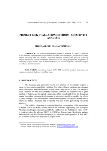
For weibull distribution, percentage change in VaR would be:withThis shows that percentage change in VaR depends on percentage change in MS, value of MF andWS probability, rather than on absolute level of MS, WS or WS/MS ratio. VaR sensitivity to MSreduces with increase in WS probability ie, sensitivity is lower for scenarios with low frequencyassociated with worst-case loss.5.1. Numerical resultsWe use a test scenario, with Median Severity of 5 million and WS of 50 Million as basecase in Year-1.Due to an improvement in risk-profile of the Bank and improvement in control environment, the Bankrevises Median severity estimate from 5 million in Year-1 to 4 million in Year-2. However, this leads toan increase in AMA capital. Conversely, an increase in Median severity due to deterioration in riskprofile would lead to a capital saving. The illustration assumes that other scenario inputs are 617371208912725597504435381OpVaR: %change frombasecase661%218%90%32%-21%-35%-45%-52%-58%5.2. VaR sensitivity to MS for different distributionsThe following chart shows VaR sensitivity to MS for three sub-exponential distributions for the aboveillustration:
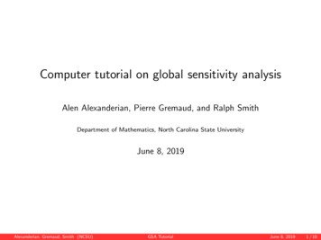
The chart below shows percentage change in VaR due to change in MS.5.3. VaR sensitivity to lower quantileThis is a generalisation of the previous results where the lower quantile is taken as the median.Scenario maybe designed in a manner such that both the quantiles are in the tail region of severitydistribution or the first quantile is in the mid region and second quantile is in the tail region. VaRsensitivity to the lower quantile is still wrong-way as shown below:
withWhere Z0 is the standard normal quantile at probability associated with lower quantile. With c’ 1, VaRwould increase due to decline in MS and vice-versa, which would be the case if frequency associatedwith worst-case scenario is greater than 0.001.Following are the practical implications of the above results: While use of SA in AMA capital models might be preferred for reasons of conservatism andforward-looking estimates, high importance to SA as direct input in AMA model may lead toundesired consequence in form of volatile capital estimate. For instance, a change in medianseverity by 1 million (from 2 million to 1 million) pushes up capital requirement by 4.04 billion.Due attention should also be given to median severity, rather than focussing solely on theworst-case severity estimates. High median severity estimates than justifiable on basis ofempirical data (internal and/or external) should be properly supported. This should be done toprevent ‘gaming’ of the scenario output.It may not be obvious to experts that for a given worst-case severity, lower median severitywould translate into higher capital and vice-versa.Banks should keep in mind that improvement/deterioration in risk profile may not have alogically consistent impact on OpVaR. This is also true for models where expert opinion iselicited for only for worst-case severity and median severity is derived from ILD. A decline isILD median would increase OpVaR and vice-versa.Choice of distribution for SA has non-trivial implications on VaR and VaR sensitivity. VaR islowest for weibull, followed by lognormal and then pareto distribution. The only exception inthe above illustration is when MS exceeds 8 million where pareto VaR declines belowlognormal VaR. It is observed that VaR sensitivity is lowest for weibull (thinnest tail), followedby lognormal and pareto distribution. For each distribution, sensitivity increases as distributiontail becomes thicker ie, with increase in shape parameter for lognormal and decline in shapeparameter for weibull and pareto.6. Right-way Sensitivity of OpVaR to Worst-case SeverityDifferentiating lognormal VaR with respect to WS, we get:Both first and second derivatives are positive for scenarios with worst-case frequency greater than0.001. This shows that OpVaR changes in same direction as worst-case severity.For ‘b%’ change in WS, percentage change in VaR for lognormal distribution would be:
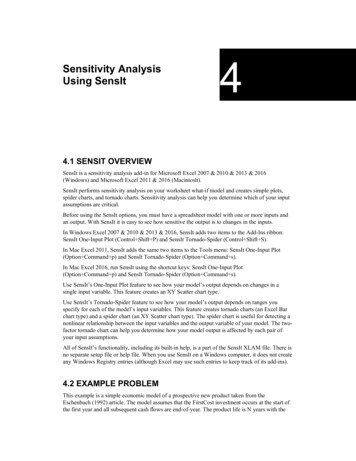
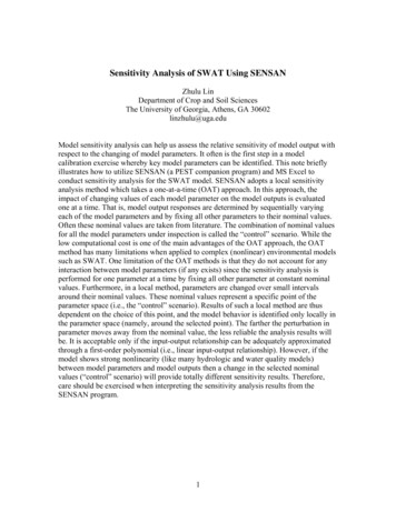
which results in:For weibull distribution, percentage change in VaR would be:withThis shows that percentage change in VaR depends on percentage change in WS, value of MF andWS probability, rather than on absolute level of MS, WS or WS/MS ratio. Further, absolutepercentage change in VaR would be greater than absolute percentage change in WS, if c 1.6.1. VaR sensitivity to WS for different distributionsVaR changes in same direction as WS for lognormal, weibull and pareto distribution. VaR and VaRsensitivity is lowest for weibull, followed by lognormal and then pareto distribution. For eachdistribution, VaR sensitivity increases as distribution tail becomes thicker.The chart below shows percentage change in VaR at different percentage change in WS.
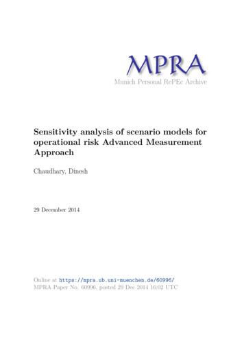
6.2. VaR sensitivity to upper quantileFollowing would be the VaR sensitivity to ‘b%’ change in upper quantile, where lower quantile may notbe the median:withWhere Z0 is the standard normal quantile at probability associated with lower quantile. With c’ 1, VaRwould increase due to increase in WS and vice-versa, which would be the case if frequencyassociated with worst-case scenario is greater than 0.001.7. VaR sensitivity to MS and WSThe following chart show impact of simultaneous change in WS and MS on VaR for three subexponential distributions.
For lognormal distribution, it maybe shown that for ‘a%’ change in MS and ‘b’% change in WS,percentage change in VaR would be:This shows that for same percentage change in MS and WS (ie, a% b%), change in VaR would alsobe a%. ie, if WS and MS are changed by a scalar such that WS/MS ratio is held constant, then VaRchanges by the same scalar. At constant WS/MS ratio, shape parameter remains constant. Therefore,VaR changes linearly with change in scale parameter. This can be shown for lognormal distributionwhere MS and WS are scaled by a scalar ‘s’, resulting in new VaR which is ‘s’ times that of existingVaR:Following chart shows VaR at various WS and MS levels such that WS/MS ratio is 10.
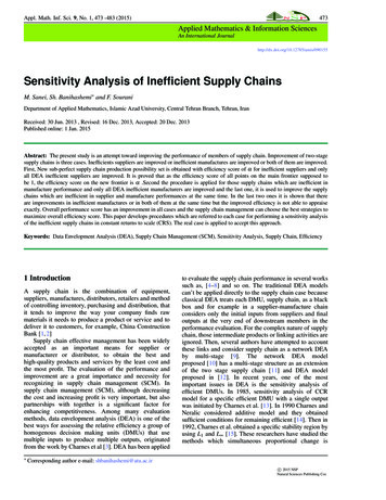
8. Wrong-way sensitivity of OpVaR to Mean Frequency for certain scenariosFor scenarios with time-based elicitation of worst-case severity, VaR is dependent on MF in twoopposing ways: MF has a direct relationship with OpVaR as VaR is the ‘MF’-fold convolution of the individualloss severity distribution.For time-based elicitation, probability associated with worst-case severity (WC probability)has direct relationship with mean frequency. Therefore, a decline (increase) in meanfrequency would result in a decline in WC probability and an increase (decline) in OpVaR.This sensitivity is not applicable for count-based scenario elicitation, as the worst-caseseverity is a pre-determined percentile of the individual loss severity distribution that does notchange due to change in MF.Indirect MF impact on VaR through ‘WC probability’ would offset the direct impact of MF on VaR,leading to wrong-way VaR sensitivity to MF. For lognormal distribution, percentage change in VaRdue to change in MF would be:whereVaR sensitivity to MF would remain same for a constant (WS/MS) ratio. Sensitivity to MF increaseswith an increase in WS/MS ratio.Illustrative results are shown below, with MF 10 considered as basecase:
Worst-caseSeverity withWCF 0.5 p.a.(Million)5050505050WC probability(1-WCF/MF)OpVaR(Million)OpvaR: %change 17%0%-34%-47%-54%Following are the practical implications of the above results: Probability associated with a worst-case loss may change due to changes in MF, even whenthe horizon associated with worst-case loss does not change. For instance, a 1 in 25 yearsththevent would be 99 quantile of severity distribution if MF is 4 and would be 96 quantile ofseverity distribution if MF is 1. Models that link scenario MF with ILD/ELD mean frequencymay exhibit logically inconsistent results over time ie, VaR may increase with decline inempirical MF and vice-versa.Linkage between MF and WS probability may not be clear to the experts during scenarioexercise. For rare events with low average arrival rate, experts’ opinion about WS may notrelate to a high quantile of severity distribution even though experts might perceive otherwise.thFor instance, a ‘1 in 25 years’ worst-case loss of 100 million would be just the 80 quantile ofseverity distribution if MF is ‘1 in 5 years’. This may lead to unrealistic capital figures forcertain rare event scenarios. Conversely, for certain ORCs a ‘1 in 2 years’ worst-case lossmaybe sufficiently in the tail if MF is very high. Therefore, for time-based elicitation it is criticalthat time horizon is carefully selected to ensure that worst-case loss is sufficiently in the tailregion.9. ConclusionThe objective of the paper was to highlight scenario model sensitivities for the benefit of practitioners.We have shown that AMA models using scenario analysis as a direct input may exhibit significantvolatility due to changes in scenario inputs. Many of the model sensitivities may not be obvious to theexperts during scenario elicitation exercise. For instance, experts might believe that lower medianseverity would result in lower capital, for same worst-case severity. Similarly, impact of a decline inmean frequency on capital due to decline in probability associated with worst-case loss may not beobvious in time-based elicitation. Another important result is that capital sensitivity increases withchoice of a conservative risk-curve for fitting to scenario data.Further work needs to be done to examine VaR sensitivity where EL term is included in the VaRapproximation and where more than two severity quantiles are elicited. Future studies are alsoneeded to examine overall capital sensitivity to scenario inputs, for models that combines scenarioand loss data using various approaches such as body-tail splice or Bayesian methods.
ReferencesBasel Committee on Banking Supervision. (2009a). Observed range of practice in key elements ofadvanced measurement approaches (AMA), 61-64Basel Committee on Banking Supervision. (2009b). Results from the 2008 loss data collectionexercise for operational risk, Annex E, 17Böcker, K. & Klüppelberg, C. (2005). Operational VAR: a closed-form approximation, Risk Magazine,90-93Böcker, K. & Sprittulla, J. (2008). Operational VAR: meaningful means, Risk Magazine, 96-98Chaudhury, M. (2010), A review of the key Issues in operational risk capital modelling, 14-19Colombo, A. & Desando, S. (2008). Developing and implementing scenario analysis models paolo.htmlOpdyke, J. & Cavallo, A. (2012), Estimating operational risk capital: The challenges of truncation, thehazards of MLE, and the promise of robust statistics, 30Risk Management Association (2012), Scenario analysis practicesRosengren, E. (2006). Operational risk scenario analysis workshop: Scenario analysis and the AMA[Powerpoint slides]. Retrieved fromhttps://www.boj.or.jp/en/announcements/release 2006/data/fsc0608be9.pdfShevchenko, P.V. & Wüthrich, M.V. (2006). The structural modelling of operational risk via Bayesianinference: combining loss data with expert opinions, The Journal of Operational Risk 1(3), 3-26
3. Scenario Generation Scenario analysis involves elicitation of expert opinions for forward-looking estimates of likelihood and impact of plausible operational risk events. Quantile approach is a common approach for scenario analysis, resulting in expert estimates for specific percentiles of the frequency and severity distribution.