Transcription
2015Quick Guide for UsingMplusESSENTIALS FOR GETTING STARTED WITH MPLUSPC USERSN. K. BOWEN, 2015
Quick Guide for Using MplusDisclaimer: Mplus is a powerful SEM program. Many options available in Mplus are notcovered here. Information on the options that are covered is based on our experiences withrecent versions of the program. These guidelines are not meant to be comprehensive orexhaustive. They reflect strategies that have worked for us. They may not reflect upcomingversions of the program or recommendations of the Mplus program developers.See also the Mplus website: http://www.statmodel.com/index.shtml for the Mplus User’s Guideprogram updates, discussion board, and other resources, and consult the in-program help feature.1
Table of Contents1 PREPARING AND SAVING DATA FILES FOR USE WITH MPLUS1a Saving Data Files for Use in Mplus1b More on Missing Values3342 SPECIFYING DATA FILES AND VARIABLES IN MPLUS SYNTAXWITH THE DATA AND VARIABLE COMMANDS AND OPTIONS2a Specifying Data Files2b Specifying Variables5563 SPECIFICYING ANALYSIS OPTIONS84 MODEL SPECIFICATION813 Examples of Mplus Syntax for Measurement and GeneralStructural ModelsExample 4.1 3-factor CFA with 9 continuous, normally distributedobserved variables, no missing valuesExample 4.2 3-factor CFA with 9 continuous, normally distributedobserved variables, and missing valuesExample 4.3 3-factor CFA with 9 continuous, normally distributedobserved variables, missing values, and two correlatedmeasurement errorsExample 4.4 3-factor CFA with 9 continuous, non-normal observedvariables, and missing valuesExample 4.5 3-factor CFA with 9 categorical observed variables, andmissing valuesExample 4.6 CFA with 9 categorical observed variables, missingvalues, and clustered dataExample 4.7 CFA with Categorical and Clustered Data, and Code forChi Square Difference Test—1Example 4.8 CFA with Categorical and Clustered Data, and Code forChi Square Difference Test—2Example 4.9 Second Order Factor ModelExample 4.10 Multiple Group CFAExample 4.11 General SEM SpecificationExample 4.12 General SEM with Latent and Observed PredictorsExample 4.13 General SEM with Latent and Observed Predictors anda Mediational Hypothesis5 MPLUS’ LANGUAGE GENERATOR99111213131415161718192122232
1 PREPARING AND SAVING DATA FILES FOR USE WITH MPLUSThis section provides information on preparing data files for Mplus. Mplus has manyoptions related to data and variables. The presentation is not exhaustive; we cover just some ofthe most common preparations social work researchers may need to make in order to have theirfiles read properly by Mplus. Mplus reads text files.Note that Mplus will save output in an output file with the same name as an input file. Ifyou change a model and want to save a new output file, save the changed input file under a newname or your original output will be over written.1a Saving Data Files for Use in MplusBefore saving an input data file, all data cleaning should be completed, any necessarydata transformations and recodes should be completed, and missing values should be recoded(see next section). Files may contain variables that will not be included in the currently plannedMplus analyses, but all variables in the text file will have to be named and listed in the Mplussyntax in order for the file to be read correctly by Mplus (more information is provided below).Mplus only reads the first 8 letters in variables names. To avoid getting a warning thatsome variable names are too long, be sure that variable names listed in Mplus syntax have 8letters or fewer.Raw data files with only numeric variables should be saved as free or fixed ASCII fileswith extensions as part of their names. They may be saved them as tab, space, or commadelimited text files. If files are saved in free format, it is not necessary to specify the file formatin Mplus syntax. Those saved in fixed format need to be described on the FORMAT line inFortran notation (e.g., F8.2). There can be no blanks in files in free format (therefore, missingvalues cannot be designated with blanks in free format text files). Files saved from SPSS as tabdelimited .dat files are among those read in Mplus. From Excel, files saved as text MS DOSfiles (with .txt extension), or “formatted text, space delimited” files (with .prn extension) areamong those that can be read.To use a lower triangle or full covariance matrix as the input matrix for Mplus, create afree format text file from a spreadsheet or database program with the matrix beginning on thefirst row of the file. To use a correlation matrix, create a free format text file that includes themeans of the variables (in the same order as they occur in the correlation matrix) on the first lineof the file, the standard deviations of the variables on the second line, and the first line of the fullor lower triangle correlation matrix on the third line.Example:1. How to format a correlation matrix of 4 variables to be used in Mplus .38Means of the four variables**Standard deviations of the four variablesCorrelation matrix of the four variables13
It is possible to create new variables from existing variables using simply arithmeticoperations once you are in Mplus, but creating recoded variables before saving your text filessaves you time later when you would have to enter the recode information in the syntax file eachtime you want to use the recoded variable.*Therefore, we recommend completing all recodes before saving your data into a text filefor use in Mplus.**We recommend using files with .txt or .dat extensions. Do not add the extensionsmanually in Windows explorer. Sometimes no extension is shown on file names listedin Windows explorer. When you add an extension manually, you are actually giving thefile a double extension (e.g., filename.txt.txt). If you add the extension manually, Mpluswill be looking for a file named filename.txt and will tell you it cannot find it because itonly sees filename.txt.txt. Find a SAVE option that creates a file with a .dat or .txtextension or, if no extension is shown, that is described as a text or dat file.**To ensure that all variables in your dataset are included in your list in Mplus and are inthe correct order, we recommend copying the full list of variables from your generalstatistics program into your buffer so it can be pasted into Mplus syntax later. Forexample, using SPSS’s pulldowns, request frequencies on all variables in the file. Pastethe syntax, copy the list of variables, and then paste it into Mplus.*1b More on Missing ValuesAs part of the preparation of data for SEM analysis in Mplus, users must designate whichsymbols or numbers in their datasets represent missing values. Options for missing valuesinclude: period (.), asterisk (*), blank (), and numeric values that are not among valid options fora variable. Because of restrictions on the use of non-numeric flags (e.g., only one per dataset),we recommend using numeric flags (e.g., 99). In addition, with data in free format, blanks andperiods may not be read correctly. Either positive or negative numeric values can be used asmissing value flags; just be sure that the value used for any one variable does not overlap with itspotential valid values. In Mplus, more than one missing flag may apply to one variable, onemissing value flag can be used for all variables, or different flags can be used to designatemissing values in different variables. Therefore, users do not have to alter existing data files tomake all missing values the same. Different treatments of variable response options can bespecified in Mplus without making changes to the original data file.Note: By default, Mplus uses a Full Information Maximum Likelihood (FIML) estimationapproach to handling missing values (if raw data are available and variables are treated asinterval level or continuous). A discussion of missing data management is beyond the scope ofthis guide, but FIML is currently a highly recommended approach (e.g., Enders, C. K., 2010,Applied missing data analysis. New York: Guilford Press). As with all missing data approaches,it assumes data are not “missing not at random.”*We recommend recoding all missing values as 99, if possible. Then, as discussed below,under the VARIABLES command in the Mplus syntax file, one simply adds “Missingare all (99).*4
2 SPECIFYING DATA FILES AND VARIABLES IN MPLUS SYNTAX WITH THEDATA AND VARIABLE COMMANDS AND OPTIONS2a Specifying Data FilesUsers specify where to find data files and what kinds of data are in data files with theDATA command and options. Note, the indentations of options under commands are for ease ofillustration; they are not required in Mplus. Mplus code lines can be continued from one line tothe next if necessary and end with a semi colon.DATA:FILE ISTYPE IS;;If a data file is not located in the same directory as the syntax file, path information isspecified in the DATA: FILE IS line. Put the full directory information inside quotation marks toavoid potential problems with spaces in directory names. See Example 1 below.If no TYPE IS line is included in the syntax, Mplus assumes the input file is in thecommon data format with one row for each subject and one column for each variable. If anotherformat is used, TYPE IS must be included in the syntax. Other TYPE IS options includeCOVARIANCE and CORRELATION for lower triangle matrices, FULLCOV and FULLCORRfor full covariance or correlation matrices, and IMPUTATION followed by a list of file names ofimputed dataset.Examples:1. The FILE IS line below indicates that the free format text file called “worksatis.dat” can befound on the D drive in the folder called “Mplus analyses.” No TYPE is specified, so it isassumed that the data file has rows for records (subjects) and columns for variables.DATA:FILE IS “D:\Mplus analyses\worksatis.dat”;2. The FILE IS line below indicates that the free format text file called “Mplustest.dat” is in thecurrent directory. The text file contains a lower triangle correlation matrix, preceded by a line(row) of means and a line of standard deviations. The third line indicates the number ofobservations (subjects) represented in the correlation matrix.DATA:FILE IS agencyinfo.dat;TYPE IS CORRELATION MEANS STDEVIATIONS;NOBSERVATIONS ARE 390;5
2b Specifying VariablesUsers indicate characteristics of their variables in the VARIABLE command section ofan Mplus input file.VARIABLE:NAMES AREUSEVARIABLES AREMISSING ARECATEGORICAL ARE;;;;The first “option” under the VARIABLE command is the required option of specifyingthe names of the variables included in the input dataset. The NAMES ARE line lists in order allthe names of the variables in the data file to be analyzed. Mplus reads text files without names,so the names entered here do not need to match any variable names used previously or displayedin other programs. Names should be 8 or fewer characters long and start with letters, but cancontain numbers and underscores. The VARIABLE: NAMES ARE line is where you could pastea list of your variables from your general statistics program instead of typing them all intoMplus.Examples:1. The NAMES ARE line in the example below indicates that the data file contains fivevariables. The USEVARIABLES ARE line indicates that only four of the five variables willbe used in the current analysis.VARIABLE:NAMES ARE gender age sowoexp typagen jobsatis;USEVARIABLES ARE age sowoexp typagen jobsatis;2. The code below specifies that all of the variables in the input data file will be included in thesubsequent modeling information. It is possible to list additional variables after ALL on theUSEVARIABLE line if new variables have been created within the Mplus program (andtherefore and not in the input file).VARIABLE:NAMES ARE gender age sowoexp typagen jobsatis;USEVARIABLES ARE ALL;The NAMES ARE and USEVARIABLES lines are critical! If the user attempts to modela variable later that was not included in the USEVARIABLES line, even if it appears in theNAMES ARE line, Mplus will return an error message. If a variable is listed in theUSEVARIABLES line and not included in the later modeling statement, Mplus will inform theuser that a variable it expected to use is “uncorrelated with all other variables.”Missing values are described in the VARIABLE command based on how they weretreated before the input data file was saved from another program. The examples below illustratehow one numeric missing value flag can be applied to all variables in a data file (Example 1),6
different variables can be assigned different missing value flags (Example 2), and each variablecan have more than one missing value flag (Example 2). Note that missing value informationonly applies to raw data files, not summary data like correlations.Examples:1. The MISSING line here indicates that for all variables, 99’s should be read as missing values.VARIABLE:NAMES ARE gender age sowoexp typagen jobsatis;USEVARIABLES ARE age sowoexp typagen jobsatis;MISSING ARE ALL (99);2. The MISSING line here indicates that missing values for variable 1 (v1) are indicated by 99,and that missing values for variable 2 (v2) are indicated by 0, 00, and 000.VARIABLE:NAMES ARE gender age sowoexp typagen jobsatis;USEVARIABLES ARE ALL;MISSING ARE v1 (99) v2 (0 00 000);One of Mplus’ strengths is its ability to appropriately analyze variables with differentdistributional and measurement qualities. The default assumption in the program is that variablesare continuous. Users can specify non-continuous variables as CENSORED, CATEGORICAL,NOMINAL, OR COUNT variables if appropriate. We focus on the second and third of thesetypes because they have been referenced throughout the book. The CATEGORICALspecification is for variables with between 2 and 10 ordered response options. CATEGORICALis the appropriate designation for observed latent variable indicators that are measured withLikesupt scale or other ordinal measures. The NOMINAL designation is used for variables withbetween 2 and 10 unordered options. Variables that are specified as either CATEGORICAL orNOMINAL are recoded by Mplus such that the response option with the lowest level becomes 0,with other options assigned higher values in increment of 1.Example:1. In the example below, the CATEGORICAL and NOMINAL lines indicate that variablesordv1 through ordv5 are what we have referred to throughout this book as ordinal variables;gender is nominal. Age is being specified by default as a continuous variable.VARIABLE:NAMES ARE gender age ordv1 ordv2 ordv3 ordv4 ordv5;USEVARIABLES ARE gender age ordv1 ordv2 ordv3 ordv4 ordv5;MISSING ARE ALL (.);CATEGORICAL ARE ordv1 ordv2 ordv3 ordv4 ordv5;NOMINAL ARE gender;7
3 SPECIFYING ANALYSIS OPTIONSThere are many analysis options in Mplus. They follow the ANALYSIS: command. Forexample:ANALYSIS:TYPE IS GENERAL:ESTIMATOR IS ML;ITERATIONS 1000;CONVERGENCE .00005;For many path models, CFA’s and general SEM’s the default TYPE IS GENERAL isadequate. As shown in the examples in the next section, however, other analysis types need to bespecified for multilevel data. The default treatment of missing values in Mplus is now FullInformation Maximum Likelihood. The default estimator is Maximum Likelihood. Similarly,there are default iteration (1000) and convergence criteria (.0005 or .00001). With a single levelpath, CFA, or general SEM, using variables that are interval level and relatively normallydistributed, all of the defaults can be used and the ANALYSIS section can be left blank.In many cases, social scientists have data that are not normally distributed or are ordinal.The examples in the next section illustrate how to request other estimators when data are notcontinuous and/or normally distributed.The Iterations value indicates how many times the program will try out sets of parameterestimates in its attempt to minimize differences between the input matrix and the matrix impliedby estimates. It is rarely necessary or useful to change the value. Most models converge with farfewer iterations, and if they don’t, more iterations are not likely to solve the problem. Theconvergence criterion is the increment of improvement in the minimization function value atwhich the program stops seeking a better model. The program is said to have converged on asolution when tweaking parameters further leads to virtually no improvement in fit.4 MODEL SPECIFICATIONModel specification occurs under the MODEL command. Here we provide annotatedexamples of a number of common types of CFA and general SEM models. Variations in theformatting of the code are presented to illustrate their equivalence. For example, “ARE,” “IS”and “ ” are equivalent. Commands can be spelled out in full or, in most cases, just the first fourletters can be provided. Annotations provide more information on syntax and options.8
13 EXAMPLES OF MPLUS SYNTAX FOR MEASUREMENT ANDGENERAL STRUCTURAL MODELSExample 4.1 3-factor CFA with 9 continuous, normally distributed observed variables, nomissing valuesMeasurement Model A. This is the CFA model specified in the measurement model examplesbelow unless otherwise p111sup21sup31com11com21com31Figure 1. Measurement Model AMplus CodeTITLE: Measurement Model of Job Satisfactionand Commitment, Continuous, NormalVariables, No Missing ValuesDATA: FILE IS "C:\Mplus\jobdata.dat";VARIABLE:NAMES AREagency sat1 sat2 sat3 sup1 sup2sup3 com1 com2 com3 age gender;USEVARIABLES ARE sat1 sat2 sat3 sup1sup2 sup3 com1 com2 com3;ANALYSIS:ESTIMATOR IS MLITERATIONS 1000;CONVERGENCE ional title is given; it will appear inoutput, which is usefulMplus reads text files; the default is freeformat, so it is not specified here.The dataset contains 12 variables.Only 9 of the variables will be used inthis analysis.ML is the default estimator; itappropriate for interval or highernormally-distributed variablesThese defaults numbers for iterations andconvergence criterion can be increased ifthe model has trouble converging.The model is a 3-factor model with 3observed indicators loading on eachfactor. “BY” indicates that JOBSATIS isbeing measured by SAT1-SAT3. LatentBY sat1 sat2 sat3 ;BY sup1 – sup3;BY com1 - com3;9
factors are named here for the first time.The observed variable names must matchthe NAMES ARE and USEVARIABLElines above.Correlations among the three factors areassumed by Mplus (default).Fully standardized parameter estimates,modifications indices that are .5 orhigher and the residual matrix arerequested. Fit indices are provided bydefault.OUTPUT: STDYX MODINDICES (.5)RESIDUAL;Note: By default, the loading of the first indicator of a factor (first variable listed after BY) isfixed at 1; covariances between pairs of exogenous latent variables are freely estimated, anderror paths are fixed at 1.To change the default setting of the first loading of JOBSATIS to 1, you make a notationin the MODEL command to free the first loading and a notation to fix an alternativeloading at 1 (here the loading of sat2 is fixed at 1). For example:JOBSATIS BY sat1* sat2@1 sat3;The “*” indicates that the default fixing of sat1’s value to 1 is changed, and the “@ 1”specifies that the loading of sat2 is fixed at 1 instead. These specifications occur in the matrix.To set the metric of JOBSATIS by fixing its variance to 1 instead of one of its loadings,similar code is used:JOBSATIS BY sat1* sat2 sat3;JOBSATIS @ 1; To change the default setting of an inter-factor correlation to 0, a “WITH” statement isadded to the model. For example:JOBSATIS WITH JOBCOMM @ 0;This code specifies that the correlation between the two factors is 0. Inter-factorcorrelations are found on the off-diagonals in the matrix.*We recommend always examining output carefully to determine if it indicates anunexpected default setting was used. Output reflects the actual parameters that were andwere not estimated. Be sure they are not different than what you intended.*10
*We recommend using the STDYX option for standardized output. It returns fullystandardized coefficients. With the STANDARDIZED option, three sets ofstandardized output are returned in the output.*Example 4.2 3-factor CFA with 9 continuous, normally distributed observed variables, andmissing valuesMplus CodeTITLE: Measurement Model of Job Satisfaction andCommitment with Continuous, NormalVariables, and Missing ValuesDATA: FILE IS "C:\Mplus\jobdata.dat";VARIABLE:NAMES AREagency sat1 sat2 sat3 sup1 sup2sup3 com1 com2 com3 age gender;USEVARIABLES ARE sat1 sat2 sat3 sup1sup2 sup3 com1 com2 com3;MISSING ARE ALL (99);ANALYSIS:TYPE IS MISSING;ESTIMATOR IS ML;ITERATIONS 1000;CONVERGENCE 0.00001;AnnotationThe missing value flag for all variablesin the current analysis is 99.The new TYPE line request thatmissing values be handled by FIML.FIML is now used by default so thisline does not need to be in the syntax.(But note that FIML cannot be usedwith summary data or categoricalvariables.)MODEL:Same as previousOUTPUT: SAMPSTATS STDYX MODINDICES(1) RESIDUAL;11Statistics on the input variables, fullystandardized parameters, modificationsindices that change by more than 1are requested, and the residual matrixare requested as output.
Example 4.3 3-factor CFA with 9 continuous, normally distributed observed variables,missing values, and two correlated measurement errorsMeasurement Model B. The CFA model specified in Example #3 has two correlatedmeasurement errors as pictured up21sup31com11com21com31Figure 2. Measurement Model BThe code for this example is the same as the code for the previous example except for theaddition of two lines to the MODEL statement. Only part of the code is presented.Mplus CodeTITLE: Measurement Model of Job Satisfaction andCommitment with Missing Values, ContinuousVariables, Two Correlated ErrorsDATA: FILE IS "C:\Mplus\jobdata.dat";MODEL:JOBSATISBY sat1 sat2 sat3 ;LIKESUPR BY sup1 – sup3;JOBCOMM BY com1 - com3;sat1 WITH sat2;com1 WITH com3;AnnotationEach factor has three observedindicators. One pair of indicators ofJOBSATIS and one pair of indicatorsfor JOBCOMM have correlatedmeasurement errors.The two “WITH” statements (in conjunction with the BY statements that specify the correlatedvariables as indicators of latent variables) specify that the two pairs of measurement errorvariances are correlated (not the variables themselves). The estimated parameters will be in the matrix.12
Example 4.4 3-factor CFA with 9 continuous, non-normal observed variables, and missingvaluesThe code for this example would be the same as the code for the models above except for achange in the ESTIMATOR option.Mplus CodeTITLE: Measurement Model of Job Satisfaction andCommitment with Non Normal ContinuousVariables and Missing ValuesDATA: FILE IS "C:\Mplus\jobdata.dat";ANALYSIS:ESTIMATOR IS MLM;ITERATIONS 1000;CONVERGENCE 0.00001;AnnotationThe MLM estimator correctsstandard errors and the chi squarestatistic for non-normality.Example 4.5 3-factor CFA with 9 categorical observed variables, and missing valuesThe code for this example is the same as the code for the models above except for changes in theVARIABLE Command and ESTIMATOR option.Mplus CodeTITLE: Measurement Model of Job Satisfaction andCommitment, Categorical Variables andMissing Values,DATA: FILE IS "C:\Mplus\jobdata.dat";VARIABLE:NAMES AREagency sat1 sat2 sat3 sup1 sup2sup3 com1 com2 com3 age gender;USEVARIABLES ARE sat1 sat2 sat3 sup1sup2 sup3 com1 com2 com3;MISSING ARE ALL (99);CATEGORICAL ARE sat1 sat2 sat3 sup1sup2 sup3 com1 com2 com3;ANALYSIS:ESTIMATOR IS WLSMV;ITERATIONS 1000;CONVERGENCE 0.00001;13AnnotationThis line indicates that the observedindicators of the latent variable arecategorical (ordinal) variables.The WLSMV estimator creates andanalyses a matrix of polychoric,tetrachoric, and/or polyserialcorrelations and an associated weightmatrix. When variables are labeled ascategorical, Mplus uses WLSMV bydefault. You cannot use FIML withsummary data, so Mplus uses apairwise deletion approach. See
Asparouhov & Muthen, 2010,“Weighted least squares estimationwith missing data,” at the Mpluswebsite for more information).MODEL:JOBSATISBY sat1 sat2 sat3 ;LIKESUPR BY sup1 – sup3;JOBCOMM BY com1 - com3;OUTPUT: SAMPSTATS STDYX MODINDICES(1) RESIDUAL;A smaller number of fit indices isavailable with WLSMV. They areprovided by default in the output.Note: This code illustrates one proper way to estimate a CFA with ordinal variables. Ifcategorical variables are specified and the ML or MLM estimator is chosen, Mplus will changethe estimator to WLSMV (and let you know with a warning in the output).Example 4.6 CFA with 9 categorical observed variables, missing values, and clustereddataTITLE: Measurement Model of Job Satisfaction andCommitment, Categorical Variables, MissingValues, and Clustered DataDATA: FILE IS "C:\Mplus\jobdata.dat";VARIABLE:NAMES AREagency sat1 sat2 sat3 sup1 sup2sup3 com1 com2 com3 age gender;USEVARIABLES ARE sat1 sat2 sat3 sup1sup2 sup3 com1 com2 com3;MISSING ARE ALL (99);CATEGORICAL ARE sat1 sat2 sat3 sup1sup2 sup3 com1 com2 com3;CLUSTER IS agency;ANALYSIS:TYPE IS COMPLEX;ESTIMATOR IS WLSMV;ITERATIONS 1000;CONVERGENCE 0.00001;MODEL:JOBSATISBY sat1 sat2 sat3 ;LIKESUPR BY sup1 – sup3;JOBCOMM BY com1 - com3;OUTPUT: STDYX MODINDICES (.5) RESIDUAL;14Don’t include agency on theUSEVARIABLES line.Data on individuals are clusteredwithin the variable “agency.” Agencyis not included in the MODELcommand; its role is specified here.With TYPE COMPLEX, standarderrors and chi square will becorrected for clustering.The categorical nature of the data ishandled by WLSMV.
Example 4.7 CFA with Categorical and Clustered Data, and Code for Chi SquareDifference Test—Step 1 (See Example 4.8 for Step 2)When users use certain estimators in Mplus, they will see the following notice under the partof the output: “The chi-square value for MLM, MLMV, MLR, ULS, WLSM and WLSMVcannot be used for chi-square difference tests.” Both the and the df are calculated differentlywith these estimators. Users will note, for example, that the df is not the difference between thenumber of unique sample moments (input covariance matrix elements) and the number ofparameters being estimated. To compare nested models when the above estimators are used inMplus requires a special process. The user cannot just compare the change in per change in df.First the user runs the less restrictive model, and includes the SAVEDATA command.TITLE: Measurement Model of Job Satisfaction andCommitment, Categorical Variables, MissingValues, Clustered Data, and DifftestSAVEDATA optionDATA: FILE IS “C:\Mplus\jobdata.dat”;VARIABLE:Same as previousANALYSIS:TYPE IS COMPLEX;ESTIMATOR IS WLSMV;ITERATIONS 1000;CONVERGENCE 0.00001;MODEL:Same as previousOUTPUT: STDYX MODINDICES (.5) RESIDUAL;SAVEDATA:DIFFTEST IS jobsat1;15With TYPE COMPLEX, standarderrors and chi square will becorrected for clustering.The categorical nature of the data ishandled by WLSMV.A small text file will be saved in theinput file directory for use by theprogram in computing the differencetest when the nested model is run.
Example 4.8 CFA with Categorical and Clustered Data, and Code for Chi SquareDifference Test—Step 2 (See Example 4.7 for Step 1)Next the user runs the nested model (with fewer parameters freely estimated than in the previousmodel). A new line is added to the ANALYSIS options.TITLE: Measurement Model of Job Satisfaction andCommitment, Categorical Variables, MissingValues, Clustered Data, and DIFFTESTAnalysis OptionDATA: FILE IS “C:\Mplus\jobdata.dat”;VARIABLE:Same as previousANALYSIS:TYPE IS COMPLEX;ESTIMATOR IS WLSMV;ITERATIONS 1000;CONVERGENCE 0.00001;DIFFTEST jobsat1;The last option under theANALYSIS command tells theprogram to use the data saved in filecreated when the first model was run,to test whether the fit of the morerestrictive (second) model issignificantly worse than the fit of thefirst.MODEL:Any model nested in previous modelOUTPUT: STDYX MODINDICES (.5) RESIDUAL;The output for the second model will include results of the difference test. If the differencehas a p value less than .05, the restrictions added to create the nested model make the fitsignificantly worse and the first model is retained. If did not become significantly worse (p .05), the second, more parsimonious, model should be retained.16
Example 4.9 Second Order Factor ModelMeasurement Model C. The diagram here shows a higher order factor “Work Experience” thatinfluences the three lower order t21sat31sup11z1sup21sup31com11com21com31Figure 3. Measurement Model CTITLE: Second Order Factor Model with CategoricalVariables and Missing ValuesDATA: FILE IS "C:\Mplus\jobdata.dat";VARIABLE:NAMES AREagency sat1 sat2 sat3 sup1 sup2sup3 com1 com2 com3 age gender;USEVARIABLES ARE sat1 sat2 sat3 sup1sup2 sup3 com1 com2 com3;MISSING ARE ALL (99);CATEGORICAL ARE sat1 sat2 sat3 sup1sup2 sup3 com1 com2 com3;ANALYSIS:ESTIMATOR IS WLSMV;ITERATIONS 1000;CONVERGENCE 0.00001;MODEL:JOBSATISBY sat1 sat2 sat3 ;LIKESUPR BY sup1 – sup3;JOBCOMM BY com1 - com3;17The new line of code names a newlatent factor and specifies that it ismeasured by the first three latent
WORKEXP BY JOBSATIS LIKESUPRfactors. The first order factorsJOBCOM;become endogenous variables.Sat1 with sat2;Com1 with com3;OUTPUT: STDYX MODINDICES (.5) RESIDUAL;Example 4.10 Multiple Group CFAA measurement model (or general SEM) can be tested to see if it is “invariant” across groups.Additional information is required in the VARIABLE, ANALYSIS, and MODEL commands.Multiple group model instructions vary depending on a number of variable and model issues.The example here is simple. A more detailed example is provided in the online book resources.Readers are also referred to the
Chi Square Difference Test—1 15 Example 4.8 CFA with Categorical and Clustered Data, and Code for Chi Square Difference Test—2 16 . Files saved from SPSS as tab delimited .dat files are among those read in Mplus. From Excel, files saved as text MS_DOS files (with .txt extension), or "formatted text, space delimited" files (with .prn .