Transcription
Unsmoothing Returnsof Illiquid AssetsSpencer Couts Andrei S. Gonçalves†Andrea Rossi‡This Version: October 2019§AbstractFunds that invest in illiquid assets report returns with spurious autocorrelation becausetheir underlying assets trade infrequently. These returns need to be unsmoothed toproperly measure risk exposures. We show that traditional unsmoothing techniquesdo not fully unsmooth the systematic component of returns, thereby understating riskexposures and overstating risk-adjusted performance. We then propose a novel returnunsmoothing method to address this issue and apply it to hedge funds and commercialreal estate funds. In doing so, we find a substantial improvement in the measurement ofrisk exposures and risk-adjusted performance. Furthermore, the improvement is greaterfor more illiquid funds.JEL Classification: G11, G12, G23.Keywords: Illiquidity, Return Unsmoothing, Performance Evaluation, Hedge Funds,Commercial Real Estate. University of Southern California, Lusk Center of Real Estate, 319 Ralph & Gold Lewis Hall, 650 ChildsWay, Los Angeles, CA 90089. E-mail: couts@usc.com.†Kenan-Flagler Business School, University of North Carolina at Chapel Hill, 4010 McColl Building, 300Kenan Center Drive, Chapel Hill, NC 27599. E-mail: Andrei Goncalves@kenan-flagler.unc.edu.‡Eller College of Management, The University of Arizona, 315P McClelland Hall, 1130 E Helen St, Tucson,AZ 85721. E-mail: rossi2@email.arizona.edu.§We are grateful for the commercial real estate data provided by NCREIF and The Townsend Group aswell as for the very helpful comments from Zahi Ben-David, Scott Cederburg, Lu Zhang, and Mike Weisbach.All remaining errors are our own.
IntroductionThe market size of intermediaries investing in illiquid assets has grown dramatically over thelast two decades.1 However, there is a lot we do not know about their risks and performancedue to the difficulty in measuring these quantities with standard techniques. Specifically, reported returns partially reflect past changes in economic values when reported and economicvalues differ due to infrequent trading and sporadic marking to market. This smoothing effect creates spurious return autocorrelation and invalidates traditional measures of risk andperformance (betas and alpha). The crux of the problem is that we only observe reported(or smoothed) returns, while we need economic (or unsmoothed) returns to evaluate risk andrisk-adjusted performance.Prior research provides different ways to recover economic return estimates by unsmoothing observed returns (e.g., Geltner (1993) and Getmansky, Lo, and Makarov (2004)). In thispaper, we argue that while previous techniques represent an important first step in measuringthe risks of illiquid assets, they do not fully unsmooth the systematic component of returns,and thus understate the importance of risk factors in explaining illiquid assets returns. Wethen provide an adjustment to return unsmoothing techniques to deal with this issue andapply our novel methodology to hedge funds and Commercial Real Estate (CRE) funds,demonstrating its usefulness in measuring the risk exposures and risk-adjusted performanceof illiquid assets. Our main finding is that systematic risk (and risk-adjusted performance) isbetter measured when returns are unsmoothed using our new return unsmoothing method.The basic idea behind return unsmoothing methods is simple. These techniques assumeobserved returns are weighted averages of current and past economic returns, estimate theseweights, and use them to recover estimates for economic returns, which are otherwise unobservable.1For instance, a report by the PwC Asset and Wealth Management Research Center shows a growth ofroughly 400% (from 2.5 trillion to 10.1 trillion) in assets under management for alternative investments(which are typically illiquid) from 2004 to 2016 (see pwc (2018)). The same report indicates that the hedgefund industry (the focus of a substantial part of our empirical analysis) has grown from 1.0 trillion to 3.3trillion over the same period.1
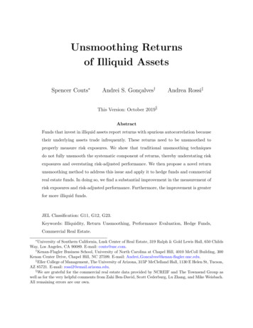
Traditional return unsmoothing techniques perform well when evaluating fund-level returns. For instance, applying Getmansky, Lo, and Makarov (2004)’s method, which is ubiquitous in the hedge fund literature, to unsmooth returns of hedge funds focused on relativevalue strategies reduces the average monthly return autocorrelation from 0.30 to 0.01. Similarly, using Geltner (1993)’s technique, which is common in the real estate literature, tounsmooth returns of CRE funds reduces the average quarterly return autocorrelation from0.72 to 0.02. These results suggest unsmoothed returns better reflect the contemporaneouschange in the true value of their underlying assets.Despite this success, we find that aggregating unsmoothed returns produces index-levelreturns that display significant autocorrelation. For instance, the monthly autocorrelationof the relative value strategy index constructed from unsmoothed hedge fund returns is still0.29. Similarly, the quarterly autocorrelation of the CRE index constructed from unsmoothedfund returns is still 0.54. These results indicate that the systematic component of fund-levelreturns is not fully unsmoothed based on traditional methods, making it difficult to properlymeasure fund risk exposures.To deal with this issue, we propose a simple adjustment to traditional return unsmoothingmethods. We assume that the observed returns of each fund are weighted averages of currentand past economic returns on both the fund and the aggregate of similar funds. We thenshow how to use a 3-step procedure to estimate the weights and obtain economic returnestimates.The 3-step unsmoothing method we propose collapses to traditional (or 1-step) unsmoothing if observed fund returns do not directly reflect lagged aggregate returns of similar funds(an underlying assumption in Getmansky, Lo, and Makarov (2004) and Geltner (1993)).However, the data do not support this assumption. Figure 1 shows (for CRE funds andhedge funds sorted on strategy illiquidity) average (normalized) coefficients from regressingfund returns on lagged fund returns and lagged aggregate returns of similar funds. Whenestimating univariate regressions in which only lagged fund returns are included, the coefficients are strong for relatively illiquid funds. Nevertheless, when lagged aggregate returns are2
0.8Coeffient on Lagged Fund Return0.7Coefficient on Lagged Aggregate yLongShortMarketNeutralGlobalMacroCTAFigure 1Regressing Fund Returns on Lagged Fund and Aggregate ReturnsThe figure plots coefficients from regressing (observed) fund returns on lagged (observed) fund andaggregate returns. The first bar for each fund category is based on a univariate regression while thesecond bar relies on a bivariate regression. Observed returns are normalized to have a unit standarddeviation so that the coefficients are comparable. The first two bars reflect real estate funds (samplefrom 1994 through 2017) while the other bars reflect different hedge fund strategies (sample fromJanuary 1995 to December 2016). See Sections 2.1 and 3.2 for further empirical details.also included in the regressions, the coefficients on lagged fund returns tend to decline, withthe coefficients on lagged aggregate returns capturing a substantial portion of the smoothingeffect. These results point to a mispecification in 1-step unsmoothing methods, and thus weapply our 3-step unsmoothing procedure to hedge funds and CRE funds.In the case of hedge funds, autocorrelation effectively disappears both at the fund-leveland strategy-level, which suggests that 3-step unsmoothing is better able to unsmooth thesystematic component of hedge fund returns than 1-step unsmoothing. Motivated by thisfinding, we explore the implications of our methodology to the measurement of risk exposuresand risk-adjusted performance of hedge funds.We perform two main exercises using hedge fund returns. In the first exercise, we sort3
funds into three groups based on the liquidity of their underlying strategy, and apply 1step and 3-step unsmoothing to funds in each of these groups. We then measure, for eachgroup, average fund volatility as well as risk and risk-adjusted performance based on astandard factor model used in the hedge fund literature (the FH 8-Factor model that buildson Fung and Hsieh (2001)). We find that volatility substantially increases after unsmoothingreturns, but the increase is roughly the same whether we use 1-step or 3-step unsmoothing.In contrast, 3-step unsmoothing produces economic returns that comove more strongly withFH risk factors (relative to 1-step unsmoothing) and display lower alphas as a consequence.The aforementioned results hold only in the low and mid liquidity groups. Unsmoothingreturns of funds in the high liquidity group has no effect on volatility, R2 s, and alphas. Thisresult indicates that unsmoothing techniques do not produce unintended distortions in theestimates of economic returns for liquid assets.In the second exercise, we repeat the analysis described above separately for funds in eachmajor hedge fund strategy category and find similar results. However, grouping funds basedon their underlying strategies allows us to study funds exposed to similar risks, and thusto explore how our 3-step unsmoothing technique improves the measurement of systematicrisk exposures. We find that our 3-step unsmoothing tends to change risk exposure estimatesin ways consistent with economic logic. For example, after unsmoothing returns using our3-step method, the exposure of emerging market funds to the emerging market risk factorstrongly increases, while other risk exposures of emerging market funds display little change.Turning to CRE funds, the overall results are similar to what we obtain with hedge funds(except that the method still leaves a portion of systematic returns unsmoothed). However,the degree to which the 3-step unsmooth process improves upon 1-step unsmoothing is muchhigher given the extreme illiquidity of real estate assets. For instance, the average beta ofprivate CRE funds to the public real estate market increases from 0.04 to 0.56, effectivelydriving the 5% annual alpha of CRE funds (measured with observed returns) to zero after3-step unsmoothing.In summary, we develop a 3-step process to improve upon traditional return unsmoothing4
techniques for illiquid assets in order to better estimate their systematic risk exposures. Wethen apply our new method to hedge funds, finding that the measurement of risk exposuresand risk-adjusted performance substantially improves after the adjustment. Finally, we perform a similar analysis based on CRE funds given their high degree of illiquidity and findthat results are even more pronounced for these funds.Our paper provides a general contribution to the literature on illiquid assets as it develops a simple way to recover economic return estimates from observed returns in orderto measure their risk and risk-adjusted performance. Several papers in this body of literature attempt to measure the illiquidity premium (e.g., Aragon (2007), Khandani and Lo(2011), and Barth and Monin (2018)). Our contribution is particularly important in thisarea because unsmoothing returns is an essential part of measuring the illiquidity premium.Without properly unsmoothing returns, any attempt to measure this premium would notcorrectly control for exposure to other sources of risk and, as a consequence, would attributethe premium associated with other risk factors to illiquidity.Our 3-step process to improve upon Getmansky, Lo, and Makarov (2004) is a significantcontribution to the hedge fund literature as it is standard practice to apply the Getmansky,Lo, and Makarov (2004) technique to unsmooth returns before studying hedge funds (e.g.,Kosowski, Naik, and Teo (2007), Fung et al. (2008), Patton (2008), Agarwal, Daniel, andNaik (2009), Teo (2009), Kang et al. (2010), Jagannathan, Malakhov, and Novikov (2010),Titman and Tiu (2011), Teo (2011), Avramov et al. (2011), Aragon and Nanda (2011),Billio et al. (2012), Patton and Ramadorai (2013), Bollen (2013), Berzins, Liu, and Trzcinka(2013), Li, Xu, and Zhang (2016), Agarwal, Ruenzi, and Weigert (2017), Gao, Gao, andSong (2018), and Agarwal, Green, and Ren (2018)).2,3 Our empirical analysis further adds2Some papers use the alternative approach of including lags of risk factors in the factor regressions (e.g.,Chen (2011), Bali, Brown, and Caglayan (2012), and Cao et al. (2013)). While useful as a quick solutionto the return autocorrelation problem, this approach does not provide a way to recover economic returnsand it dramatically increases the number of parameters to be estimated in the factor regressions, which isan important limitation as investors often face the problem of measuring multiple risk exposures based on arelatively short time-series.3While we interpret our results from the lens of illiquidity, misreporting can also induce smoothed returns(Bollen and Pool (2008, 2009) and Aragon and Nanda (2017)). We do not attempt to disentangle the two5
to previous papers in the hedge fund literature by demonstrating that hedge fund alphas arelower than previously recognized, once systematic risk is properly measured using our 3-stepunsmoothing method.We also contribute to the real estate literature because we show that our unsmoothingtechnique can be used to improve upon the autoregressive unsmoothing method in Geltner(1993), which is commonly applied in the real estate literature (e.g., Fisher, Geltner, andWebb (1994), Barkham and Geltner (1995), Corgel et al. (1999), Pagliari Jr, Scherer, andMonopoli (2005), Rehring (2012), and Pagliari Jr (2017)).Our improvement upon traditional unsmoothing techniques reaches beyond the hedge fundand real estate literatures, however. For instance, unsmoothing methods have been appliedto other types of illiquid funds such as private equity, venture capital, and bond mutual funds(Chen, Ferson, and Peters (2010) and Ang et al. (2018)), to highly illiquid assets such ascollectible stamps and art investments (Dimson and Spaenjers (2011) and Campbell (2008)),and even to unsmooth other economic series such as aggregate consumption (see Kroencke(2017)).The rest of this paper is organized as follows. Section 1 introduces the traditional, 1step, return unsmoothing framework and develops our 3-step unsmoothing process to improve upon it; Section 2 applies 1-step and 3-step unsmoothing to hedge fund returns anddemonstrates that the latter improves upon the former in measuring risk exposures and riskadjusted performance; Section 3 extends the analysis to CRE funds; and Section 4 concludes.The Internet Appendix provides supplementary results.1A New Unsmoothing MethodAcademics and practitioners rely primarily on two methods in order to obtain economic (orunsmoothed) returns, Rt , from observed (or smoothed) returns, Rto . These methods can besources of return smoothness because, when considering the perspective of an investor or econometricianattempting to estimate economic returns, the degree of return smoothness is the relevant variable, not thesource of smoothness. Moreover, Cassar and Gerakos (2011) and Cao et al. (2017) find that asset illiquidityis the major driver of autocorrelation in hedge fund returns.6
used to unsmooth illiquid asset returns or returns of funds that invest in illiquid assets, butwe refer to returns as belonging to funds for concreteness since, in our empirical analysis, weunsmooth returns of hedge funds and commercial real estate funds.Both unsmoothing methods assume Rto is a weighted average of current and past Rt ,but the two techniques differ in how the weights are specified. The first method, developedby Getmansky, Lo, and Makarov (2004), leaves weights unconstrained, but requires a finitenumber of smoothing lags (we refer to this framework as MA unsmoothing as it impliesa moving average time-series process for Rto ). The second method, developed by Geltner(1993), allows for an infinite number of smoothing lags, but constrains weights to decayexponentially (we refer to this framework as AR unsmoothing as it implies an autoregressivetime-series process for Rto ). The former method is mainly used in the hedge fund literaturewhile the latter is applied more generally to unsmooth returns of highly illiquid assets andits most common application is in the real estate literature.We refer to the Getmansky, Lo, and Makarov (2004) (MA) and Geltner (1993) (AR)methods generally as “1-step unsmoothing” and develop a 3-step approach (for both MAand AR) that improves upon 1-step unsmoothing methods. Subsection 1.1 details the 1step MA unsmoothing method; Subsection 1.2 demonstrates that it does not fully unsmooththe systematic portion of returns; and Subsection 1.3 develops our 3-step MA unsmoothingtechnique to address this issue. The description of the AR unsmoothing framework is providedin Section 3, where we also unsmooth returns of commercial real estate funds.1.1The 1-step MA Unsmoothing MethodTable 1 provides the basic characteristics of the hedge funds we study (the data sourcesand sample construction are detailed in Subsection 2.1). There are 10 different hedge fundstrategies (sorted by the average fund-level 1st order return autocorrelation coefficient) witha total of 4,827 funds and an average of 89 monthly returns per fund. Hedge funds display(annualized) average excess returns varying from 2.3% to 5.7% and (annualized) Sharperatios varying from 0.22 to 0.60, with more illiquid funds displaying higher Sharpe ratios.7
It is well known that some hedge fund strategies rely on illiquid assets, and thus theobserved returns of hedge funds may be smoothed. To deal with this issue, Getmansky, Lo,and Makarov (2004) (henceforth GLM) propose a method to unsmooth hedge fund returns.GLM assume the observed return of fund j at time t is given by (see original paper for theeconomic motivation):4(0)(1)(H)oRj,t θj · Rj,t θj · Rj,t 1 . θj· Rj,t Hj(1)(h) µj Σ Hh 0 θj · ηj,t h(2)(h)where θs represent the smoothing weights with ΣHh 0 θj 1 and the second equality followsfrom GLM’s assumption that Rj,t µj ηt,j with ηj,t IID.The first equality represents the economic assumption that the observed fund return is aweighted average of the fund’s economic returns over the most recent H 1 periods, includingthe current period. The second equality is an econometric implication that says that, underthe given assumption, the observed fund returns follow a Moving Average process of orderH, MA(H).Given Equation 2, we can recover economic returns by estimating an MA(H) processofor observed returns, Rj,t, extracting the estimated residuals, ηj,t , and adding the estimatedexpected return, Rj,t µj ηj,t . GLM also provide the basic steps to estimate θs by maximumiid2likelihood under the added parametric assumption that ηj,t N (0, ση,j).5 This procedure isused by several papers in the hedge fund literature to unsmooth returns (e.g., Kosowski, Naik,and Teo (2007), Fung et al. (2008), Patton (2008), Agarwal, Daniel, and Naik (2009), Teo(2009), Kang et al. (2010), Jagannathan, Malakhov, and Novikov (2010), Titman and Tiu(2011), Teo (2011), Avramov et al. (2011), Aragon and Nanda (2011), Billio et al. (2012),4The fact that H does not depend on j simplifies the notation but does not imply the number of MAlags is not fund dependent. Specifically, letting Hj represent the number of MA lags with non-zero weight(h)for fund j, we define H max(Hj ) and set θj 0 for any h Hj .5The method is almost identical to the one used in most statistical/econometric packages. The only(0)difference is that statistical/econometric packages tend to impose the normalization θj 1 as opposed to(h)ΣHh 0 θj 1. To translate from the first to the second normalization, one needs to divide the coefficients(1)(H)estimated by the package (and multiple the estimated residuals) by 1 θj . θj8.
Patton and Ramadorai (2013), Bollen (2013), Berzins, Liu, and Trzcinka (2013), Li, Xu,and Zhang (2016), Agarwal, Ruenzi, and Weigert (2017), Gao, Gao, and Song (2018), andAgarwal, Green, and Ren (2018)).We apply the 1-step MA unsmoothing to each hedge fund in our dataset using the AICcriterium to select the number of MA lags (allowing for H from 0 to 3 months). Table 2contains the (average) autocorrelations (at 1, 2, 3, and 4 lags) for hedge fund returns (observed and unsmoothed) as well as the % of funds with a significant autocorrelation at 10%level. Observed returns display relatively high autocorrelations. For instance, relative valuefunds have average 1st order autocorrelation of 0.30, with 65.1% of these funds displayingstatistically significant autocorrelations. After 1-step MA unsmoothing, average autocorrelations are basically zero at all lags and the % of funds displaying statistically significantautocorrelations is in line with the statistical error of the test.The results indicate that 1-step MA unsmoothing produces economic returns that arelargely unsmoothed at the fund level. This correction is important to properly analyse hedgefunds because smoothed returns understate volatilities and betas, and thus overstate Sharperatios and alphas, as demonstrated by GLM.1.2Implications to Aggregate Fund ReturnsUnder the central assumption of unsmoothing methods, we should also observe strategyindex returns that are not autocorrelated. Specifically, for any set of time-invariant weights,wj , the assumption that Rj,t µj ηt,j with ηj,t IID implies:Rt ΣJj 1 wj · Rj,t ΣJj 1 wj · µj ΣJj 1 wj,t · ηj,t µ ηt(3)where η t IID, which means that Et 1 [Rt ] µ (i.e., aggregate returns are unpredictable,and thus they should not be autocorrelated).Table 3 shows autocorrelations for each (equal-weighted) strategy index. Reported returns9
display quite high autocorrelations. For instance, the relative value strategy has a 1st orderautocorrelation of 0.51 (statistically significant at 1%). The autocorrelation coefficients remain high after aggregating unsmoothed returns. For instance, the relative value strategy stillhas an autocorrelation of 0.29 (statistically significant at 1%) after 1-step MA unsmoothing.The results suggest that 1-step unsmoothing delivers strategy indexes with substantialautocorrelation, which indicates that the approach used by the previous literature to unsmooth returns does not fully unsmooth the systematic component of returns. This result isimportant because if the systematic portion of returns is not fully unsmoothed, then betasestimated after traditional unsmoothing will be understated and alphas overstated, whichhas non-trivial implications for performance analysis.1.3The 3-step MA Unsmoothing MethodWe develop a 3-step unsmoothing procedure to addresses the issue raised in the previoussubsection. The basic idea is to obtain unsmoothed returns as the sum of unsmoothed aggregate returns and unsmoothed excess returns, where the aggregate and excess returns areunsmoothed separately.We refer to the “aggregate” of a generic variable, yj,t , as y t ΣJj 1 wj · yj,t and its “excess”as yj,t y t , where wj are arbitrary (but time-invariant) weights with ΣJj 1 wj 1. Moreover,we keep the total number of funds, J, constant over time while developing our aggregationresults.This subsection relies on the fact that, for arbitrary variables xj and yj,t , we have:6ΣJj 1 wj · xj · yj,t x · y t ΣJj 1 wj · (xj x) · (yj,t y t )d j , yj,t ) x · y t Cov(x6(4)This result is a generalization of the typical covariance decomposition for the case of non-equal weights:ΣJj 1 wj · (xj x) · (yj,t y t ) ΣJj 1 wj · xj · yt,j y t · ΣJj 1 wj · xj x · ΣJj 1 wj · yt,j x · y t · ΣJj 1 wj ΣJj 1 wj · xj · yt,j x · y t10
We generalize the underlying assumption in Equation 1 so that aggregate economic returnscan be directly used in the smoothing process:7(h) e(h)LoRj,t ΣHh 0 φj · Rj,t h Σh 0 πj · Rt h(h)(5)(h) µ j ΣHej,t h ΣLh 0 πj · η t hh 0 φj · η(6)ej Rj,t Rt are excess returns, η and ηewhere Rt ΣJj 1 wj · Rj,t are aggregate returns, R(h)(h)Lare the respective shocks, and the weights add to one, ΣHh 0 φj Σh 0 πj 1.In GLM, the weights on past economic returns, θs, add to one to assure that information(h)is eventually incorporated into observed prices. Our restriction, ΣHh 0 φj(h) ΣLh 0 πj 1,has the same effect.Aggregating Equation 6 yields:oRt µ π (0) · η t π (1) · η t 1 . π (L) · η t Hd (0) , ηej,t ) Cov(φd (1) , ηej,t 1 ) . Cov(φd (H) , ηej,t H ) Cov(φjjj µ ΣLh 0 π (h) · η t h(7)where the first equality relies on Equation 4 and the second equality is based on a larged (h) , ηej,t h ) Cov(φ(h) , ηej,t h ) 0. The restricsample approximation that uses P lim Cov(φjjJ (h)tion ΣLh 0 πj 1 assures the aggregate moving average parameters satisfy ΣLh 0 π (h) 1 sothat aggregate information is eventually incorporated into aggregate prices.8Subtracting Equation 7 from Equation 6, we have observed excess returns:eo ΣH φ(h) · Rej,t h ΣL ψ (h) · Rt hRj,th 0 jh 0 j(h)(h) µej ΣHej,t h ΣLh 0 ψj · η t hh 0 φj · η7(8)This smoothing process reduces to Equation 1 (the 1-step unsmoothing process in GLM) if we set(h)(h) φj θj . Moreover, as in the 1-step method, the fact that H and L do not depend on j simplifiesthe notation but does not imply the number of MA lags is not fund dependent. Specifically, letting Hj and Ljrepresent the number of MA lags with non-zero weight for fund j, we have H max(Hj ) and L max(Lj )(h)(h)with φj 0 for any h Hj and πj 0 for any h Lj .(h)(h)(h)8J ΣL ΣJj 1 wj · (ΣLSince ΣLh 0 πh 0 Σj 1 wj · πjh 0 πj ) 1(h)πj11
(h)where ψj(h)(h) πj π j .Equations 7 and 8 provide a simple way to recover aggregate and fund-level economicreturns in an internally consistent way. First, we get aggregate economic returns fromoRt µ η t where η t are residuals of a MA(H) fit to Rt . Second, we obtain fund-level ecoej,t µnomic excess returns from Rej ηej,t where ηej,t are residuals from a MA(H) fit (witheo .9 Third, we recover fund-level economic returns fromη t , η t 1 , ., η t L as covariates) to Rj,tej,t µj η t ηej,t . This procedure summarizes our 3-step unsmoothing proRt,j Rt Rcess.10(h)Note that if πj(h) φj , which is the main assumption in GLM (our Equation 1), then:(h)(h)(h)oej,tR µej ΣHej,t h ΣH) · η t hh 0 φj · ηh 0 (φj φo(h) µ j ΣHh 0 φj · ηj,t h Rt(9)so that our method is equivalent to recovering ηt directly from the residuals of a MA(H) fite o R o µj R o µj .to Rj,ttj,tConsequently, our 3-step procedure can be seen as a generalization of GLM that allowsaggregate and excess economic returns to have different effects on observed fund-level returns(h)(π j(h)6 φj ), but recovers precisely the same unsmoothing procedure if the underlying(h)(h)assumption in GLM (π j φj ) is imposed.The last four columns of Tables 2 and 3 show the results from our 3-step unsmoothingprocess. From Table 2, unsmoothed fund-level returns display autocorrelations comparableto the ones obtained from 1-step unsmoothing. In contrast to 1-step unsmoothing, how9As in the 1-step method, if the aggregate and fund-level MA processes are estimated by standard(0)statistical packages (which would normalize π (0) 1 in step 1 and θj 1 in step 2), then we need to dividethe coefficients estimated by the package (and multiple the estimated residuals) by 1 π (1) . π (L) in(1)(H)(h)the Step 1 and by 1 φj . φj in Step 2. The ψj coefficients do not need to be adjusted in step 2.10Step 2 of the 2-step method requires the estimation of a MA(H) with η t , η t 1 , ., η t L as covariates toaccount for the influence of aggregate returns into the fund-level unsmoothing process. One way to further(h)(h)simplify the procedure would be to assume πj π (h) since this assumption implies ψj 0 (i.e., nocovariates in the MA process for observed excess returns). In Internet Appendix A, we report results underthis more restrictive structure. There is little change in the 3-step method’s performance under this extra(h)restriction. However, we do not impose the restriction πj π (h) in the main text to allow for the realisticfeature that the unsmoothing processes of different funds depend differently on aggregate returns.12
ever, Table 3 shows that our 3-step unsmoothing method effectively drives strategy-levelautocorrelations to basically zero.11 As such, the 3-step approach properly unsmoothes thesystematic portion of returns, which has important economic consequences explored in thenext section.2Unsmoothing Hedge Fund ReturnsIn this section, we unsmooth hedge fund returns to demonstrate that our 3-step unsmoothing technique improves upon traditional unsmoothing in terms of measuring risk and riskadjusted performance of funds that invest in illiquid assets. Subsection 2.1 explain the empirical details; subsection 2.2 presents the main results after separating funds into liquidity-basedgroups; and subsection 2.3 reports results by hedge fund strategy to explore the improvementin risk measurement.2.1Empirical Details(a) Hedge Fund DatasetWe combine data from two major commercial hedge fund databases to build our hedgefund dataset. Specifically, we merge the Lipper Trading Advisor Selection System database(hereafter TASS), accessed in June 2018, with the BarclayHedge database, accessed in April2018, which produces a representative coverage of the hedge fund universe.12 Both dataproviders started keeping a so-called graveyard database of funds that stopped reportingtheir returns only in 1994. Hence, following the literature, we start our analysis of fund risk11Strategy-level returns from the 3-step unsmoothing method are obtained by aggregatingRt,j µj η t ηej,t
†Kenan-Flagler Business School, University of North Carolina at Chapel Hill, 4010 McColl Building, 300 Kenan Center Drive, Chapel Hill, NC 27599. E-mail: Andrei Goncalves@kenan-flagler.unc.edu. ‡Eller College of Management, The University of Arizona, 315P McClelland Hall, 1130 E Helen St, Tucson, AZ 85721. E-mail: rossi2@email.arizona.edu.