Transcription
Illiquid Homeownership and the Bank of Mom andDad*Job Market PaperNovember 24, 2020 (Link to most recent version)Eirik Eylands Brandsaas AbstractHousing is the largest asset in U.S. households’ portfolios but parentaltransfers are important for housing outcomes. How much of the homeownership rate among young households is accounted for by parental transfers? Ibuild and estimate a life-cycle overlapping generations model with housing, inwhich children and parents interact without commitment. I find that parentaltransfers account for 15 percentage points (31%) of the homeownership rateof young adults. Transfers from wealthy parents increase homeownership byrelaxing borrowing constraints and reducing housing risk. Policies and regulations that decrease the sales cost of housing increase homeownership andweaken the link between parent wealth and housing outcomes. Finally, I studyhow housing illiquidity affects the commitment frictions between parents andchildren. Children with wealthy parents increase their consumption of illiquidhousing to extract larger future transfers.*Ihave benefited from the comments of Dean Corbae, Erwan Quintin, Ananth Seshadri, Corina Mommaerts, Paul Goldsmith-Pinkham, Tim Kehoe, Manuel Amador, Hamish Low, PatrickMoran, and Joel McMurry, as well as participants at the 19th Annual Society for the Advancementof Economic Theory Conference (SAET), Oxford NuCamp Macro Workshop, Young EconomistSymposium 2020 at University of Pennsylvania, Minnesota-Wisconsin Macro/International Workshop and various seminars at University of Wisconsin-Madison. I gratefully acknowledge financialsupport from the Norwegian Finance Initative. University of Wisconsin-Madison. E-mail: eebrandsaas@gmail.com1
1IntroductionHousing is the largest asset in US households’ portfolios and among middle-classhouseholds represents the primary means of wealth accumulation. There are growingconcerns about housing affordability and inequality in access to housing. One contributing factor to inequality in housing outcomes is parental transfers. Around 30%of American first-time homebuyers received downpayment assistance from parentsin 2009-2016. Parental downpayment assistance averaged 48,000 among receivinghouseholds.1 Owner-occupied housing bears adjustment costs that make it illiquid.In addition, households must meet a downpayment requirement to obtain a mortgage. These two frictions, transaction costs and credit constraints, increase the importance of transfers for homeownership. First, transfers directly alleviate borrowingconstraints. Second, future transfers decrease the probability that households haveto sell their house after experiencing adverse income shocks. Third, illiquid housingacts as a commitment device that the child uses to extract future transfers.In this paper, I ask: how much of the homeownership rate among young (2544) households is accounted for by parental transfers? In addition, I quantify howmuch different financial and housing regulations affect the link between parentalwealth, transfers, and their children’s housing outcomes. Finally, I study how housingilliquidity affects the commitment problem between children and parents.To answer these questions, I merge the literatures on models of housing, whichignore transfers, with models of parental transfers, which ignore housing. I build alife-cycle overlapping generations model with altruistic parents and a rent or own decision. Children and parents interact, without commitment, through both inter-vivostransfers and bequests at death from the parent. My key innovation to the altruismframework is to include illiquid housing, which interacts with transfers. In modelswithout housing (e.g., Boar, 2018; Altonji, Hayashi, and Kotlikoff, 1997; Barczyk and1Data from the Survey of Household Economic Decisionmaking and the Transfer Supplement ofthe 2013 Panel Study of Income Dynamics (see Section 2).2
Kredler, 2014), the only transfer motive is to increase the child’s goods consumptionwhen they are up against a borrowing constraint. Illiquid housing introduces twoadditional transfer motives. First, young adult children enter the economy with lowwealth and low income and they must save to buy a house. Parents, who are atthe life-cycle peak of wealth and income, may choose to transfer money to alleviate minimum downpayment requirements. Second, children who own a house andexperience income losses may avoid costly downsizing by receiving parental transfers. Moreover, children can extract future transfers from their parents by shiftingliquid wealth to illiquid housing (“house-rich, cash-poor”). On the other hand, as inall models of transfers, future transfers decrease the savings motive, decreasing thehomeownership rate.I estimate the model by matching data on homeownership, savings, and transfersfrom the Panel Survey of Income Dynamics (PSID). I then compute a counterfactualhomeownership rate by simulating the model without parental transfers. Withoutparental transfers, the model collapses to a standard life-cycle model with housing.I find that parental transfers account for 15 p.p. (32%) of the young homeownershiprate. Two frictions, a minimum downpayment requirement and an adjustment coston housing, account separately for 77% and 61% of the parental transfer effect onhomeownership, respectively. In the benchmark model the supply of owner-occupiedhousing is perfectly elastic, but my results are robust to other supply elasticities. Iuse my model to quantify the contribution of parental transfers to the black-whitehomeownership gap: in the US young white households are twice as likely to behomeowners as black households. I find that parental transfers account for 30% ofthe black-white homeownership gap.After documenting that parental wealth and transfers are an important determinant of homeownership I study how policies that increase homeownership also affectthe link between parental wealth and children’s housing outcomes. Decreasing minimum downpayments strengthens the link between parental wealth and children’s3
housing outcomes since households with wealthy parents find homeownership moreattractive. Increasing liquidity, by decreasing sales and purchase costs, weakens thelink between parental wealth and children’s housing outcomes by reducing the riskof ownership which is more important for households with poorer parents. Finally, Istudy how housing illiquidity affects the strategic behavior introduced by the lack ofcommitment. I find that 13% of young households prefer to face sales costs as theycan reduce liquid wealth by over-investing in housing and thus extract larger futuretransfers. On the other hand, sales cost increase precautionary savings motives, andso households with less wealthy parents save more, decreasing the need for futuretransfers.By introducing parental transfers to models of housing, my paper contributes tothe literature studying the determinants of homeownership over the life-cycle. Recentpapers focus on marriage and family formation (Fisher and Gervais, 2011; Chang,2020; Khorunzhina and Miller, 2019), housing demand in old-age (McGee, 2019; Barczyk, Fahle, and Kredler, 2020), and changing borrowing constraints (Paz-Pardo,2019; Mabille, 2020). These studies highlight the importance of credit constraintsand minimum down payments in constraining demand for owner-occupied housing.However, by considering parent-child interactions, I show a dichotomy based on parent wealth in the importance of constraints. For households with poorer parents, thesales and purchase costs decrease ownership by it riskier to own. This risk is less important for households with richer parents making mortgage credit constraints moreimportant. My results highlight that policies that increase ownership by subsidiesto first-time buyers will lead to increased housing inequality.I contribute to the growing literature that studies altruistic households who interact without commitment by studying how illiquid housing affects the commitmentproblem. In these models children undersave to increase parental transfers (e.g., Altonji et al., 1997; Boar, 2018; Barczyk and Kredler, 2014). However, adjustment costson housing impose future expenditure commitments (Chetty and Szeidl, 2007; Shore4
and Sinai, 2010). I show that expenditure commitments have two distinct effectson child-parent interactions. First, the child can buy a house and bring no liquidwealth to the next period. If the parent does not give a transfer, the child must sellhis house and pay adjustment costs or decrease consumption drastically. A wealthyaltruistic parent likes neither of these outcomes and responds by transferring. Second, by giving gifts that push the child to buy the parent makes future undersavingmore expensive since the child cannot easily sell his house. Both mechanisms arequantitatively meaningful. First, 17% of 25-year old households prefer their housing to be illiquid to extract future transfers. Second, illiquid housing increases thechild-parent wealth ratio from 0.09 to 0.11.Finally, I contribute to the literature on parental transfers and life-cycle outcomesby focusing explicitly on how parental transfers to young adult households changetheir savings choices through homeownership. My results show that households withwealthier parents are willing to buy sooner, take higher leverage, and need to holdless liquid precautionary savings. My results highlight how parental wealth increasesthe persistence of wealth inequality by affecting household risk-taking. Previousliterature has generally studied parental investment in their children’s human capital(e.g., Lee and Seshadri, 2019; Daruich, 2018) or transfers from adult children toretired parents (e.g., Mommaerts, 2016; Barczyk and Kredler, 2018; Barczyk et al.,2020), instead of the effect of parental wealth on household portfolio choices.The paper proceeds as follows. In Section 2, I describe the data sources, summary statistics, and document that parental wealth is associated with better housingoutcomes. Section 3 describes the quantitative model and Section 4 discusses thestructural estimation. Section 5 performs the main quantitative exercise and robustness tests. Finally, Section 6 studies how policies intended to increase homeownershipalso affect the role of parent wealth and housing illiquidity.5
2Data on Transfers, Family, and HousingI first present the estimation sample, taken from 1997-2017 waves of the Panel Studyof Income Dynamics (PSID). I also use two other surveys to discuss the time trendsin the reliance on parental transfers for house down payments. Finally, I use theestimation sample to show that parental wealth is positively associated with betterhousing outcomes.2.1Panel Study of Income DynamicsThe primary data source is the Panel Study of Income Dynamics (PSID), whichfollows a nationally representative sample of US households and their descendantsover time since 1968. The PSID is the only publicly available US dataset that satisfiesthis paper’s three requirements. First, it has detailed wealth, income, and housingdata for both parents and adult children. Second, it has some information aboutinter-vivos transfers from parents to children. Third, it follows households over time,so we can observe the transitions from renting to owning and how the transitionrelates to parental wealth.I use data from 1999 to 2017. In 1999 the PSID started to collect detailed wealthdata every other year. In most waves of the PSID, there is limited transfer data, andthe main question is whether households received gifts or bequests over 5,000 dollarsin the last two years. In 2013 the PSID collected more detailed transfer data in theFamily Roster and Transfer Module. They asked parents how much they gave theirchildren in the last calendar year and how much they had given over their lifetimefor school, house purchases, or other purposes. Household characteristics such asage, gender, and education refer to the household head. I classify top-coded valuesas missing observations. All monetary variables are expressed in constant 2016 USdollars (in thousands).Sample Selection: Throughout this paper, the sample includes all households6
aged 25-84 in the PSID, excluding the Survey of Economic Opportunity and theLatino sub-samples to obtain a representative sample. All summary statistics arecalculated using the provided family weights.Matching Parents with Children: I use the Parent/Child file from the PSID’s2013 transfer supplement. I can observe each household’s reported transfers to andfrom parents and children. This leads to discrepancies, where the child and parentdoes not agree on the amount given from the parent to the child. I only use theparent’s reported transfer. First, there may be some stigma about receiving transfers,which may induce receiving children to under-report. Second, in the model, parentsdetermine the size of the transfer they give to their child. I treat each parent-childpair as separate so that two siblings with the same parent household are counted astwo independent households.Definition of Transfers: The 2013 transfer supplement asks all parent householdswhether they gave money, gifts, or loans of 100 or more to their children in 2012.There is no identifying information on whether these transfers are gifts or loans,and I treat all as gifts.2 Since this paper focuses on transfers that are a) related tohousing and b) quantitatively meaningful, I set transfers below 500 to 0.32.2Descriptive Statistics: Who Receives Transfers?I now discuss descriptive statistics from the PSID sample in 2013 for householdsaged 25-44 with a non-missing parent household. Tables 1 and A4 contain the sample means and medians, broken down by age, wealth, marriage, house tenure, andwhether households received transfers in the last year. In panel a), the first twocolumns compare the whole sample, broken down by whether they received transfersor not in the last calendar year. The mean transfer is relatively high at 3,940,2While transfers may be given as a loan, we know that parental loans are often not-repaid, areinterest-free, and are loans in name only.3Ignoring small transfers decreases the transfer rate from 32% to 24% and increases the meantransfer from 2,921 to 3,944.7
and 27% of households received transfers in the last year. Both groups have similarwealth levels, but transferring parents are much wealthier, with a median wealth of 339,000 relative to non-transferring parents who had 96,860. Recipients are morelikely to be college-educated, white, and a little younger. Receivers are somewhatless likely to be homeowners (39% vs. 43%).By breaking down the sample by marital status, we see that married or cohabitinghouseholds are wealthier, have higher household income, are more likely to be white,slightly older, and have approximately three times the homeownership rate of singlehouseholds. Married households are somewhat more likely to receive transfers andreceive slightly larger transfers. Next, I break the sample down by whether they arerenting or owning. Homeowners have ten times the wealth of renters and also havesignificantly wealthier parents. There is no difference between renters and ownersin the receipt rates, but transfers to owners are on average 1,000 larger. Only 6%of renters owned in the previous period, while 21% of owners rented in the previousperiod. Further, receivers are more likely to switch from renting to owning: 21% ofreceiving owners rented two years ago, compared to 15% of non-receiving owners.Next, I break the sample into five age groups from 25-44. We see that household’swealth, income, and homeownership rates increase with age. As households becomewealthier they are less likely to receive transfers. Interestingly, owners are morelikely to receive transfers than renters: among households aged 29-32, 32% of nonreceivers and 40% of receivers were homeowners. Not only are those who receivedmore likely to own, they are also likelier to be new homeowners: Only 13% of owningnon-receivers are new homeowners, compared to 21% of owning receivers.8
Table 1: Descriptive Statistics (Means), Households Aged 20-44AllReceiverNoYesTransfer0.003.94Wealth78.41 108.33Wealth Parent 404.94 5Owner0.430.39Owner th Parent 320.86 3Owner0.190.16Owner t-20.140.14Age26.4926.49Observations572195Wealth QuintileReceiverQuintile 1NoYesTransfer0.00Wealth-53.90Wealth Parent r nterNoYesOwnerNoYes0.003.4930.7156.93325.54 2.7931.4510943040.004.49126.76 171.11485.26 1016.5699.69 103520.003.9113.4242.02241.36 2.2231.3314534000.004.00163.53 210.84619.05 1048.00106.65 125629-32No33-36Yes0.004.1237.6378.53379.41 0.4830.45566163Quintile 88975.38102.730.390.890.590.5342.4072Quintile .048.25559.6246.190.400.810.160.2231.29121Quintile 4NoYesQuintile 5NoYes0.005.2939.9742.02391.03 4.1733.144711370.004.95339.67 403.71938.08 2046.24131.73 8159Notes: Data from the PSID Transfer, Individual, and Family modules. Weighted using family weights. Transfer,wealth, and income measured in 1000s of 2016 USD.9
Finally, I break down the sample by wealth quintiles. Within each wealth quintile,receivers and non-receivers have virtually identical wealth, income, and age. Still, receivers are slightly more likely to be white and college-educated within each quintile.The largest difference is that the receiver’s parents are much wealthier. We also seethe clear inter-generational correlation of wealth: Parents with children in the topquintile have four times the wealth of parents with children in the bottom quintile.I now briefly summarize the main results. In 2013, 27% of young householdsreceived a transfer, and transfers averaged 3,940. Receivers have significantly richerparents, have similar wealth and income as non-receivers, and are less likely to own.Receiving transfers increases the probability of transitioning from renting to owning,especially in the age groups where households are most likely to buy. Parents’ wealthis strongly correlated with the probability of receiving a transfer.2.3Parental Transfers for Owners Over TimeFrom the PSID transfer supplement, we have seen how those who receive transfers differ from their counterparts in 2012. Two additional data sources show thatparental transfers for housing have increased over the last two decades.Survey of Household Economics and Decisionmaking (SHED): To better understand US households’ financial health, the Federal Reserve first conducted the SHEDin 2013. It is an annual cross-sectional survey with a focus on financial well-being.In 2015 and 2016, the survey asked homeowners when they bought their home andhow they funded the downpayment.4 The results are plotted in the left panel of Figure 1. The main observation is the large increase in the role of inter-vivos transfersfor homeowners since 2001. In 2001-2007, only 5-18% of first-time buyers receivedtransfers, while 20-40% received transfers after 2009.In 2013, 2014, and 2016 the SHED contained a question asking renters why4The data were recorded for owners who bought since 2001 in the 2015 wave and those whobought since 2015 in the 2016 wave.10
Figure 1: Increased Reliance on Parental Transfers for Down PaymentsRecieved Gifts/Loan For DownpaymentMostly Gifts/Inheritance for ear of Purchase200020102020Survey YearNotes: The left panel uses data from the SHED. First-time homeowners are defined as thosewho did not use proceeds from previous property sales for the downpayment. Bars indicate 95%confidence intervals. The right panel uses data from the public AHS file. The patterns are differentsince the horizontal axis is different and that the AHS sample includes all owner-occupied units.they rent. The main barrier to homeownership was borrowing constraints: 57% ofUS households mentioned that they could not afford a down-payment or did notqualify for a mortgage. In addition to borrowing constraints, the survey revealsthat illiquidity the associated with owner-occupied decreases homeownership: 26%mentioned that renting was more convenient and 23% that planning to move asreasons for renting.American Housing Survey: I use the AHS to obtain a time series back to 1991.The AHS follows roughly 60,000 housing units over time and asks households inowner-occupied units how they funded the downpayment (right panel of Figure 1).We see a relatively flat trend in the ’90s, followed by a quick decline in 2005-2008 asmore households were using mortgages with low down payments. Finally, we see adramatic increase in the years after the housing bubble. The horizontal axis denotesthe survey year and not the year of purchase. Small changes thus indicate largechanges among new owners who are a small subset of all owners.11
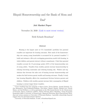
2.4Hypothesis I: Households With Wealthier Parents AreLess Likely To DownsizeIf parent wealth provides insurance, households with wealthier parents should beless likely to downsize after income losses. I perform an event study on the effect ofunemployment on housing consumption to test this hypothesis.The sample is limited to household heads who are unemployed only once betweenages 25 and 45. The consumption value of owner-occupied housing is set to 6% of themarket value as in Boar, Gorea, and Midrigan (2020). For renters, I use the rentalpayment. The log growth rate is defined as the difference in log housing consumptionbetween t and t 2. Households who switch between renting and owning are codedas missing.5 I use parental wealth as a proxy for transfers since transfers were onlyobserved in 2013. I divide the sample by whether a household’s parents were in thetop parental wealth quartile at the time of unemployment.I then compare the housing consumption responses when households become unemployed by parental wealth to examine whether households with wealthier parentsare less likely to downsize. The results are displayed in Figure 2. Households withnon-wealthy parents decrease the growth rate of housing consumption from 4% to6%, a significant change at the 5% level. Households with parents in the top 25%have no statistically significant decrease in housing consumption growth rates. Moreover, I replicate this event study using simulated data from the quantitative modeland show that the results are similar (see Section 4.4 and Figure 4).5This methodology is inspired by Chetty and Szeidl (2007) who find that housing consumptionresponds less to unemployment than non-durable consumption, as predicted by a model with illiquidhousing. I focus on showing that parental wealth supports a household’s housing consumption.Further details are in Appendix A.2, where I also report results separately for renters and owners.I report results from the event study with control variables in Appendix A.2.1, and the results arequantitatively similar.12
Figure 2: Event Study: Housing Consumption at Unemployment by Parental WealthHousing Growth RateHousing Growth RateParents in Bottom 75%.2.10-.1-.2-4-2024Parents in Top 25%.2.10-.1-.2-4Years Relative to Unemployment-2024Years Relative to UnemploymentNotes: Solid lines denote means, and bars denote the 95% confidence interval. Sample consists ofhouseholds aged 25-45 with exactly one unemployment spell and without changes in head and/orspouse in the four years before and after unemployment.2.5Hypotheses II: Parental Wealth Affects House PurchasesThe previous results provide strong evidence that parent wealth provides insuranceagainst downsizing after income losses. I now show that households with wealthierparents also buy more expensive houses and are less likely to be behind on mortgagepayments, controlling for household characteristics.2.5.1Households With Wealthier Parents Buy Larger HousesI run an ordinary least square (OLS) regression on house values at purchase for firsttime buyers and test whether parent’s wealth is positively associated with largerhouse purchases, controlling for net worth, income, education, age, family size, andrace:ln HouseSizei β1 ln(W ealth)p(i),t 2 β2 ln(Incomei,t 2 ) β3 ln(N etW orthi,t 2 ) γXi,t εi ,Parent’s wealth, as well as household income and net-worth, are logged. Householdsare denoted by i, their parents by p(i), and Xi , t denotes a vector of controls includingtime, age, education, state and race dummies.Column 1 of Table 2 reports the results from an OLS regression of house values13
among first-time buyers. We can see that households with wealthier parents buylarger houses: A 1% increase in parental wealth is associated with a 0.042% increasein the purchase value of the child’s house. The effect of parental wealth is almost aslarge as that own the child’s own net worth (0.068%).2.5.2Households With Wealthier Parents Are Less Likely to Have Mortgage DifficultiesI now show that households with wealthier parents are less likely to be behind ontheir mortgages, even though they buy more expensive houses. Since 2009 the PSIDhas collected information on whether households are behind on their mortgages. Thepercentage of households behind on mortgage payments has decreased from 3.8% in1999 to 1.8%. Overall, 8.6% of the sample have been behind at least once. Thisresult stresses that parental transfers relax borrowing constraints and also reducethe downsides of illiquid housing. Households who take out large mortgages andcannot follow the payment plan may be behind on mortgage payments, ultimatelyending in foreclosure. Being behind on mortgage payments is an indicator of financialstress and is typically expensive due to fees. I now measure whether parental wealthdecreases households’ probability of being behind on mortgage payments, controllingfor demographic variables.I perform OLS regressions of the following form:EverBehindi β1 ln(W ealth)p(i),t 2 β2 ln(Incomei,t 2 ) β3 ln(N etW orthi,t 2 ) γXi,t εi ,where the sample is limited to the first time a household is observed as owners.In column (2) of Table 2, I report results when the outcome variable is whetherhouseholds are ever behind on mortgage payments, and we see that parental wealthin the period before purchase decreases the probability that a household will ever bebehind: A 1% increase in parent wealth decreases the probability of being behind14
Table 2: Housing Choices and Parental WealthParentWealth (t-2)Child HouseholdNet Worth (t-2)Income (t-2)High School 1College 1White 1Family SizeN(1)House Size(2)Ever Behind(3)Behind First(4)Behind RE(5)Behind FE0.052 (0.019)-0.019 (0.008)-0.022 (0.007)-0.008 (0.004)-0.007(0.009)0.068 (0.015)0.309 (0.033)0.260 (0.067)0.538 (0.078)0.056(0.057)0.094 34(0.036)-0.057 (0.027)0.027(0.021)-0.013 (0.007)0.017(0.013)-0.074 (0.032)-0.064 (0.036)0.035(0.023)0.008(0.019)-0.008 2,0572,057Notes: Standard errors in parentheses. ‘Behind’ refers to whether the households is behind on amortgage. Wealth, income, parental wealth, mortgage, family size, and house values are logged.All regressions include year and state fixed effects and control for age and age-squared of both thechild and parent. Specifications 1-3 uses ordinary least squares while specifications 4 and 5 userandom and fixed effects, respectively.15
by 0.019 percentage points, and is significant at the 1% level. The effect of parentalwealth is larger than the effect of the child’s net worth but smaller than the effect ofthe child’s income. In Column (3) the outcome variable is whether households arebehind in the first period, and we see coefficients and significance levels are virtuallyunchanged.I also report the results from two specifications where I follow the same households as in Column (2) after purchase. I report results from random effects andhousehold fixed effects regressions in Columns (4) and (5), respectively. Once wefollow households over time, the effect of parental wealth decreases. With householdfixed effects the effect is no longer significant. However, the FE regressions must beinterpreted with caution since there is little time variation in parental wealth withina family. Indeed, the random effects and the fixed effect coefficient are almost thesame (0.007 vs 0.008). Overall, the results support the hypothesis that parentalwealth decreases the probability of being behind on mortgage payments.3A Quantitative Model of Family Banking andHousingThis section describes my life-cycle model of housing choices with overlapping generations, idiosyncratic earnings risk, and altruistic inter-vivos transfers from parentsto children (“kids”). The model has two main building blocks. The first is altruism and no commitment. Parents are altruistic towards their children and deriveutilit
liquid wealth to illiquid housing (\house-rich, cash-poor"). On the other hand, as in all models of transfers, future transfers decrease the savings motive, decreasing the homeownership rate. I estimate the model by matching data on homeownership, savings, and transfers from the Panel Survey of Income Dynamics (PSID). I then compute a .