Transcription
Multivariable Calculus with MaximaG. Jay KernsDecember 1, 2009The following is a short guide to multivariable calculus with Maxima. It loosely followsthe treatment of Stewart’s Calculus, Seventh Edition. Refer there for definitions, theorems,proofs, explanations, and exercises. The simple goal of this guide is to demonstrate how touse Maxima to solve problems in that vein.This was originally written for the students in my third semester Calculus class, but onceit grew past twenty pages I thought it might be of interest to a wider audience. Here it is. Iam releasing this as a FREE document, and other people are free to build on this to makeit better. The source for this document is located athttp://people.ysu.edu/ gkerns/maxima/It was inspired by Maxima by Example by Edwin Woollett, A Maxima Guide for CalculusStudents by Moses Glasner, and Tutorial on Maxima by unknown. I also received help fromthe Maxima mailing list archives and volunteer responses to my questions. Thanks to all ofthose individuals.Contents1 Getting Maxima1.1 How to Install imaxima for Microsoft Windowsr . . . . . . . . . . . . . . . .1.1.1 Install the software . . . . . . . . . . . . . . . . . . . . . . . . . . . .1.1.2 Configure your system . . . . . . . . . . . . . . . . . . . . . . . . . .2 Three Dimensional Geometry2.1 Vectors and Linear Algebra . . . .2.2 Lines, Planes, and Quadric Surfaces2.3 Vector Valued Functions . . . . . .2.4 Arc Length and Curvature . . . . .3 Functions of Several Variables3.1 Partial Derivatives . . . . . . . . . . . .3.2 Linear Approximation and Differentials .3.3 Chain Rule and Implicit Differentiation .3.4 Directional Derivatives and the Gradient1.4455.6681419.2023242527
3.53.6Optimization and Local Extrema . . . . . . . . . . . . . . . . . . . . . . . .Lagrange Multipliers . . . . . . . . . . . . . . . . . . . . . . . . . . . . . . .4 Multiple Integration4.1 Double Integrals . . . . . . . . . . . . . . . . . . .4.2 Integration in Polar Coordinates . . . . . . . . . .4.3 Triple Integrals . . . . . . . . . . . . . . . . . . .4.4 Integrals in Cylindrical and Spherical Coordinates4.5 Change of Variables . . . . . . . . . . . . . . . . .2932.3333343435365 Vector Calculus5.1 Vector Fields . . . . . . . . . . . . . . . . . . . . . . . . . . . . . . . . . . .5.2 Line Integrals . . . . . . . . . . . . . . . . . . . . . . . . . . . . . . . . . . .5.3 Conservative Vector Fields and Finding Scalar Potentials . . . . . . . . . . .373739416 Miscellaneous6.1 Saving your plots . . . . . . . . . . . . . . . . . . . . . . . . . . . . . . . . .6.2 Saving your Maxima commands . . . . . . . . . . . . . . . . . . . . . . . . .4343447 GNU Free Documentation License452.
Copyright c 2009 G. Jay KernsPermission is granted to copy, distribute and/or modify this document under the terms ofthe GNU Free Documentation License, Version 1.3 or any later version published by the FreeSoftware Foundation; with no Invariant Sections, no Front-Cover Texts, and no Back-CoverTexts. A copy of the license is included in the section entitled “GNU Free DocumentationLicense”.3
1Getting MaximaThere are many ways to get Maxima, and the choices are governed somewhat by the user’soperating system (although Maxima proper is platform independent). The home page forMaxima (which has links to download from SourceForge) ishttp://maxima.sourceforge.netThis document was written with Emaxima on GNU-Emacs. Emacs is a powerful texteditor, and Emaxima uses Emacs to integrate Maxima input/output with LATEX code toproduce documents that look like they could have come from a textbook. That’s why themathematical expressions below are so pretty. See the following link to learn more ModeIf you do not want to write a paper but just want to work with Maxima interactivelythen another option is imaxima, which also works with Emacs and LATEX (and Ghostscript) totypeset Maxima input/output professionally. To learn more about imaxima see the h/Another option that exists is TeXmacs, but I do not have much experience with it. Fromwhat I can gather it has a good reputation.1.1How to Install imaxima for Microsoft WindowsrThe following instructions are to set up imaxima on a computer with a Microsoft Windowsroperating system (the majority of users). If you are running Mac-OS then instead go ad-and-install/easy-install-on-mac-os-x,and if you are running Linux (like me) you can go ad-and-install/easy-install-on-linux.Please note that these instructions are NOT needed to install plain-old Maxima. Itis already installed in Cushwa 1062, and you can install it at home with the ’Maxima’instructions in the next subsection.4
1.1.1Install the softwareIn order to take advantage of the full power of imaxima you need several things.MiKTEX 2.7 (pronounced “MICK - teck”) is an up-to-date implementation of TEX andrelated programs for Windowsr. Its official web site is www.miktex.org. You can goto http://www.miktex.org/2.7/Setup.aspx and click the Download button of theBasic MiKTeX 2.7 Installer on that page. You may save the .exe file anywhere,such as the Desktop. Start the installation with a double-click. You need to install itin the default place.GPL Ghostscript 8.63 The main page for Ghostscript is http://www.cs.wisc.edu/ ghost/.To download the latest Ghostscript 8.64 compiled for Windowsr, you go tohttp://pages.cs.wisc.edu/ ghost/doc/GPL/gpl864.htm.In the middle of the page there there is a link to the file you need. Choose gs864w32.exe(or the latest release; if you have a 64-bit system then you will need gs864w64.exe,and if you do not know what I am talking about then you probably do not need the64-bit version). You can double click the downloaded gs864w32.exe file to start theinstallation. You need to install it in the default place.Maxima Go to http://sourceforge.net/projects/maxima/files/, and scroll down tothe Maxima-Windows section. Choose maxima-5.19.2.exe (or the latest release) for thedownload of a Windowsr pre-compiled binary installer. Double click the downloadedmaxima-5.19.2.exe file to start installation. You need to install it in the default place.Emacs is a very powerful text editor. The very official precompiled release can be obainedfrom http://ftp.gnu.org/pub/gnu/emacs/windows/. However, the distributed precompiled binary does NOT support image features, hence it is not good enough forimaxima, by default. Thanks to Vincent Goulet, however, you can obtain a precompiled binary installer which has everything you need to use imaxima. Go to the webpage indows and chooseemacs-23.1-modified-3.exe for download. Just follow the instructions and install itin the default place.1.1.2Configure your systemOnce you have installed all of the above, go to the Start Menu under GNU Emacs and clickUpdate Site Configuration. In the file that opens add the following single line (and it has tobe exactly right) to the top of the file and click the Save button. Note that there shouldn’tbe any line break; it is one, big, long, line.( load " C :/ Program Files / Maxima -5.19.2/ share / maxima /5. 19.2/ emacs/ setup - imaxima - imath . el ")If you have installed a different version of Maxima then the 5.19.2 appearing twice inthe above line should be replaced with the version you have downloaded.Then quit Emacs and restart. When it opens, type:5
M - x imaximaThe symbol M means the Alt key (which is also known as the Meta key). Thus, thecommand M-x imaxima means1. Hold down the Alt key and press x.2. Let go, then type imaxima, then press Enter.If this is your first time using imaxima, MikTEX will probably ask you to install the mhpackage from CTAN. Please proceed with Yes for installation. This may take some time, sobe patient.Then, you will see the initial screen of Maxima. Enjoy!!2Three Dimensional Geometry2.1Vectors and Linear AlgebraWe set up vectors in a way which is slightly different from how we do it in Maple.(%i1)(%o1)a: [1,2,3];[1, 2, 3](%i2)(%o2)b: [2,-1,4];[2, 1, 4]We can do the standard addition and scalar multiplication of vectors.(%i3)(%o3)3 * a;[3, 6, 9](%i4)(%o4)a b;[3, 1, 7]The dot product operator is a simple period "." between the vectors.(%i5)a . b;6
(%o5)12We can check our answer to make sure it is right.(%i6)(%o6)1 * 2 2 * (-1) 3 * 4;12To do cross products we must load a special package, the vect package, which is includedwith a/5.19.2/share/vector/vect.macThe symbol for the cross product is the tilde " " up on the left corner of the keyboard(you need to do Shift to get it).(%i8)(%o8)a b;([1, 2, 3] , [2, 1, 4])(%i9)(%o9)express(%);[11, 2, 5]The cross product did not look like anything at the beginning; we had to express thecross product to get something recognizable.The norm (length) of a vector is the square root of the dot product of the vector withitself.(%i10)(%o10)sqrt(a . a); 147
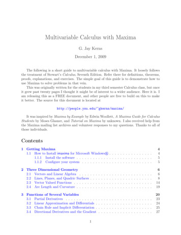
Putting what we have learned all together we may do vector projections and scalar tripleproducts (we will need another vector c for the STP to make sense).(%i11)(%o11)(a . b)/(a . a) * a; (%i12)(%o12)6 12 18, ,7 7 7 c: [-5, 2, 9];[ 5, 2, 9](%i13)(%o13)a . (b c);[1, 2, 3] · ([ 2, 1, 4] , [5, 2, 9])(%i14)(%o14)express(%); 96Again, we needed to express the cross product to get anything useful.2.2Lines, Planes, and Quadric SurfacesWe can plot planes with implicitplot from the draw package.First let us define the plane with equation3x 4y 5z 0.We store the equation of the plane in the variable plane1.(%i1)(%o1)plane1: 3*x 4*y 5*z 0;5z 4y 3x .2/share/draw/draw.lisp(%i3)(%o3)draw3d(enhanced3d true, implicit(plane1, x,-4,4, y,-4,4, z, -6,6));[gr3d (implicit)]8
64624200-2-2-4-6-4-6-4-3-2-101234 -4-3-2-101234Figure 1: A plot of a planeLet us next plot an ellipsoid with equationx2 y 2 z 2 3.3We plot it just like we plot the plane.(%i4)(%o4)ellips1: x 2/3 y 2 z 2 3;z2 y2 (%i5)(%o5)x2 33draw3d(enhanced3d true, implicit(ellips1, x,-3,3, y,-2,2, z, -2,2));[gr3d (implicit)]We can also use Maxima to help us find an equation of a plane based on defining vectors.For instance, let’s find and plot the plane determined by the points A(1, 1, 1), B(1, 2, 3), andC(0, 0, 0).First we define the position vectors for the three defining points.(%i6) a: [1, 1, 1];(%o6)[1, 1, 1]9
23 -2-1.5-1-0.500.511.52Figure 2: A plot of an ellipsoid(%i7)(%o7)b: [1, 2, 3];[1, 2, 3](%i8)(%o8)c: [0, 0, 0];[0, 0, 0]Next, we find the vectors from A to B, and A to C.(%i9)(%o9)ab: b - a;[0, 1, 2](%i10)(%o10)ac: c - a;[ 1, 1, 1]Then, we find the normal vector to the plane. (Recall that we need the vect package todo cross products.)(%i11)load(vect);10
vect.mac(%i12)(%o12)n: express(ab ac);[1, 2, 1]Finally, we set up the defining equation of the plane, which takes the formn · r n · r0 .(%i13)(%o13)r: [x, y, z];[x, y, z](%i14)(%o14)r0: a;[1, 1, 1](%i15)(%o15)plane: n . r n . r0;z 2y x 0The only remaining task is to make the plot. See Figure BLANK.(%i16)(%o16)draw3d(enhanced3d true,implicit(plane,x,-4,4,y,-4,4,z,-4,4));[gr3d (implicit)]We can do more exotic plots, like cones. Let’s do a standard cone with equationx2 y 2 z 2(%i17)(%o17)cone: x 2 y 2 z 2;y 2 x2 z 2(%i18)draw3d(enhanced3d true, implicit(cone, x,-1,1, y,-1,1, z,-0.5,0.5));11
43210-1-2-3-443210-1-2-3-4-4-3-2-101234 -4-3-2-101234Figure 3: Another plot of a 0.5-0.500.51 -1Figure 4: A plot of a cone12
.511.52 -2-1.5-1-0.500.511.52Figure 5: A plot of a hyperboloid(%o18)[gr3d (implicit)]See Figure BLANK. See how the center of the cone looks distorted? It is because weare plotting the cone in rectangular coordinates. We get a much better plot with sphericalcoordinates. More on that later.Let’s next try a hyperboloid with equationx2 y 2 z 2 1See Figure BLANK.(%i19)(%o19)hyperboloid: x 2 y 2 - z 2 1; z 2 y 2 x2 1(%i20)(%o20)draw3d(enhanced3d true, implicit(hyperboloid, x,-2,2, y,-2,2, z,-1.5,1.5));[gr3d (implicit)]And we can do a hyperboloid of two sheets, with the equation x2 y 2 z 2 1.13
-0.500.511.52 -2-1.5-1-0.500.511.52Figure 6: Another plot of a hyperboloidSee Figure BLANK.(%i21)(%o21)hyprbld2: -x 2 - y 2 z 2 1;z 2 y 2 x2 1(%i22)(%o22)draw3d(enhanced3d true, implicit(hyprbld2, x,-2,2, y,-2,2, z, -2,2));[gr3d (implicit)]2.3Vector Valued FunctionsWe define vector functions in Maxima just like we would any other function; the only difference is that the return value is a vector.(%i1)(%o1)r(t) : [t, cos(t), sin(t)];r (t) : [t, cos t, sin t]Once we have the function we can plug in values of t to evaluate.(%i2)r(1);14
0.80.60.40.20-0.2-0.4-0.6-0.8-1 -0.8-0.6 -0.4-0.200.2 0.40.6 0.8-0.2-0.4-0.6-0.81 -100.80.60.40.21Figure 7: A space curve in 3-d(%o2)[1, cos 1, sin 1](%i3)(%o3)float(%);[1.0, .5403023058681398, .8414709848078965]Now let’s try some plotting. Let’s first try a space curve of the vector function. We needthe draw package to make this happen. Once we have it loaded, we do space curves with theparametric function inside of a draw ametric(cos(t), -cos(t), sin(t), t, -4, 4));[gr3d (parametric)]See Figure 1. Sometimes the line width of a space curve leaves something to be desired.We can fix the issue with the line width argument to the draw command. See Figure 2.15
Limits of vector functions operate just like limits of everything else. Notice below howto do limits from the right and left.(%i6)(%o6)limit(r(t), t, 2);[2, cos 2, sin 2](%i7)(%o7)float(%);[2.0, .4161468365471424, .9092974268256817](%i8)(%o8)limit(r(t), t, 2, plus);[2, cos 2, sin 2](%i9)(%o9)limit(r(t), t, 3, minus);[3, cos 3, sin 3]Derivatives of vector-valued functions are, again, just like their one-valued counterparts.(%i10)(%o10)diff(r(t), t);[1, sin t, cos t]We need to be careful, here. In both Maple and Maxima the return value of diff(r(t),t)is an expression, and is NOT a function (although it sure does look like one). Looks aredeceptive in this case. Watch what happens if we try to use it like a function.(%i11)(%o11)wrong(t) : diff(r(t),t);wrong (t) : diff (r (t) , t)(%i12) wrong(1);** error while printing error message ** :M: second argument must be a variable; found M#0: wrong(t 1)– an error. To debug this try debugmode(true);This is not right. The way to get around this in Maple is to do D(r(t),t), and the wayto get around this in Maxima is to do the following.16
(%i13)(%o13)define(rp(t), diff(r(t), t));rp (t) : [1, sin t, cos t]Now we get what we expect.(%i14)(%o14)float(rp(1));[1.0, .8414709848078965, .5403023058681398]We may define the unit tangent vector T as the normalized derivative of r. We do thiswith the uvect function in the eigen ect(rp(t));(%i17)(%o17)trigsimp(%);1sin tcos tp, p,p(sin t) 2 (cos t) 2 1(sin t) 2 (cos t) 2 1(sin t) 2 (cos t) 2 1 (%i18)(%o18)1sin t cos t , , 222 define(T(t), %); sin t cos t1T (t) : , , 222 To get the unit normal vector we need to get the derivative of T and normalize.(%i19)(%o19)define(Tp(t), diff(T(t), t)); cos t sin tTp (t) : 0, , 2217 #
(%i20)(%o20)uvect(Tp(t));"(%i21)(%o21)0, pcos t(sin t) 2 (cos t) 2trigsimp(%);, psin t(sin t) 2 (cos t) 2#[0, cos t, sin t](%i22)(%o22)define(N(t), %);N (t) : [0, cos t, sin t]Now we find the binormal vector, B, by calculating the cross product of T and N.Remember to do load(vect) if you haven’t already during the ss(T(t) N(t)); (%i25)(%o25)(sin t) 2 (cos t) 2 sin t cos t , , 2222trigsimp(%); (%i26)(%o26)1 sin t cos t , , 222 define(B(t), %); 1 sin t cos tB (t) : , , 222(%i27)(%o27) float(B(1));[.7071067811865475, .5950098395293859, .3820514243700898]18
2.4Arc Length and CurvatureThere is no special Maxima function for the curvature but we can do it with the formulaswe learned in class. Recall from the last section that r(t) ht, cos t, sin ti and1sin t cos tT(t) , , .222with derivative′T (t) (%i1)(%o1)r(t)cos tsin t0, , 22.: [t, cos(t), sin(t)];r (t) : [t, cos t, sin t](%i2)(%o2)rp(t) : [1 ,-sin(t), cos(t)];rp (t) : [1, sin t, cos t](%i3)(%o3)Tp(t) : [0, -cos(t), sin(t)]/sqrt(2);Tp (t) : (%i4)(%o4)sqrt(Tp(t) . Tp(t))/sqrt(rp(t) . rp(t));q(%i5)(%o5)[0, cos t, sin t] 2trigsimp(%);(sin t)22 (cos t)22p(sin t) 2 (cos t) 2 112(%i6)(%o6)define(kappa(t), %);κ (t) : 12We have a lot of practice with derivatives, but we can integrate, too.(%i7)integrate(r(t), t);19
(%o7) t2, sin t, cos t2With integrals we can compute the arc length, but be warned, the arc length may only*rarely* be calculated in closed form. More often than not the arc length can not be represented by an elementary function. We do an example for the sake of argument. We will definea simple vector function, calculate the derivative, and integrate the norm of the derivative.(%i8)(%o8)g(t) : [2 * t, 3 * sin(t), 3 * cos(t)];g (t) : [2 t, 3 sin t, 3 cos t](%i9)(%o9)define(gp(t), diff(g(t), t));gp (t) : [2, 3 cos t, 3 sin t](%i10)(%o10)integrate(trigsimp(sqrt(gp(t) . gp(t))), t, 0, 2*%pi); 2 13 πNote that we used the special notation %pi for our favorite mathematical constant. Weneed the same thing for Euler’s constant %e and the imaginary unit %i.Also note that we wrapped sqrt(gp(t) . gp(t)) with trigsimp in the integratecall. As of the time of this writing, there is a bug in Maxima so that the integral is notcomputed correctly without the simplification. See Bug ID: 2880797 in the Maxima bugtracker.Especially with arc lengths sometimes we need to do numerical integration instead ofsymbolic integration. We can do it with the romberg function.(%i11)(%o11)romberg(sqrt(gp(t) . gp(t)), t, 0, 2*%pi);22.654346798277953Functions of Several VariablesNow let’s try some multivariate functions.(%i1)f(x,y) : (x 2 - y 2) 2;20
8070605040302010032-31-20-10-112-23 -3Figure 8: A plain surface plot of a function of two variables(%o1)f (x, y) : x2 y 2 2Let’s take a look at a it(f(x,y), x, -3, 3, y, -3, 3));[gr3d (explicit)]See Figure BLANK.The important part is to enclose the function with explicit(). We can get a fancier,colored plot if we put enhanced3d true at the beginning of the function call.(%i4)(%o4)draw3d(enhanced3d true, explicit(f(x,y), x, -3, 3, y, -3, 3));[gr3d (explicit)]We can see level curves (also known as a contour map) of the function f with the following:21
2-23 -3Figure 9: An enhanced surface plot of a function of two variables(%i5)draw3d(explicit(f(x,y), x, -5, 5, y, -5, 5),contour levels 15,contour map);(%o5)[gr3d (explicit)]An alternative is to use(%i6)(%o6)contour plot(f(x,y), [x, -5, 5], [y, -5, 5] );falseThe contour map is a 2D plot. If we raise the contour lines up to the plot surface thenthe lines are more precisely called horizontal traces. Here is a plot of r levels contour surface hide true,x, -3, 3, y, -3, 3),15,surface,true);(%o7)[gr3d (explicit)]22
igure 10: A contour plot, showing level curves of f .See Figure 6. We do surfacehide true so that we can see the traces better.3.1Partial DerivativesWe do partial derivatives in the natural way. For example, for the partial derivative withrespect to x we do(%i1)(%o1)diff(f(x,y), x);df (x, y)dxThe long way to get higher order derivatives is to nest the diff calls. The second orderpartial derivative is(%i2)(%o2)diff(diff(f(x,y), x), x);d2f (x, y)d x2and the second partial with respect to x then y is(%i3)diff(diff(f(x,y), x), y);23
0032-31-20-10-112-23 -3Figure 11: Another form of contour plot which shows horizontal traces on f(%o3)d2f (x, y)dxdyFor higher order partial derivatives a quicker way is to do(%i4)(%o4)G: x 7 * y 8;x7 y 8(%i5)(%o5)diff(G, x, 1, y, 2, x, 3);47040 x3 y 6The above first differentiates G with respect to x three times, then with respect to ytwo times, and finally with respect to x one time; that is, the arguments match the Leibnitznotation for partial derivatives.3.2Linear Approximation and DifferentialsA function of two variables is differentiable at a point (x0 , y0 ) when it is closely approximatedby the tangent plane to the curve at (x0 , y0 ). We saw in class how to find the tangent plane24
at (x0 , y0 ), and we also discussed how we could use the tangent plane to approximate valuesof f (x, y) for (x, y) near (x0 , y0 ).We will not bother with the tangent plane in Maxima, but we can quickly find the linearapproximation L to f (which is essentially the same thing) by means of the taylor function.2Let f (x, y) ex sin(y) and let us find the linear approximation of f at the point (1, 2).(%i1)(%o1)f(x,y) : exp(x 2) * sin(y);f (x, y) : exp x2 sin y(%i2)(%o2)taylor(f(x,y), [x,y], [1,2], 1);sin 2 e (2 sin 2 e (x 1) cos 2 e (y 2)) · · ·The function L is shown in the output as everything but the three dots. The ellipsis is away to indicate that the returned expression is an approximation to the original function.The linear approximation arguments are all self explanatory except the last. It representsthe order of the Taylor series. When we find a linear approximation to a differentiablefunction what we are actually doing is finding a Taylor series of order 1, about the point(x0 , y0 ).We can get the total differential by doing diff without specifying any independentvariables.(%i3)(%o3)diff(f(x,y));22ex cos y del (y) 2 x ex sin y del (x)The symbols del(y) and del(x) stand for dy and dx, respectively.3.3Chain Rule and Implicit Differentiation2Suppose we have a function of two variables, f (x, y) ex sin y.(%i1)(%o1)f(x,y) : exp(x 2) * sin(y);f (x, y) : exp x2 sin yWe saw earlier what the partial derivatives of f were with respect to x and y. Butsuppose x and y are functions of some other variables, for instance,(%i2)[x,y] : [s 2 * t, s * t 2];25
(%o2) 2 s t, s t2Then what are the partial derivatives of f with respect to s and t? Happily for us,Maxima does the chain rule automatically.(%i3)(%o3)diff(f(x,y), s);4 s3 t2 es(%i4)(%o4)4 t2diff(f(x,y), t);2 s4 t es4 t2 4 2sin s t2 t2 es t cos s t2 4 2sin s t2 2 s t es t cos s t2That was easy. But be warned that the derivative with respect to x does not workanymore.(%i5) diff(f(x,y), x);** error while printing error message ** :M: second argument must be a variable; found M– an error. To debug this try debugmode(true);We could fix this by using different letters, u and v:(%i6)(%o6)diff(f(u,v), u);22 u eu sin vBut that is cheating. A better way to fix it is to kill the relationship between x and s, t.(%i7)(%o7)kill(x, y);done(%i8)(%o8)diff(f(x,y), x);22 x ex sin y26
Implicit differentiation is relatively easy, given what we have already done. For example,let’s find the first partial derivatives of z when xyz x2 y 3 z 4 x xz.(%i9)(%o9)F: x*y*z x 2*y 3*z 4 - x - x*z;x2 y 3 z 4 x y z x z x(%i10)(%o10)Fx: diff(F, x);2 x y3 z4 y z z 1(%i11)(%o11)Fy: diff(F, y);3 x2 y 2 z 4 x z(%i12)(%o12)Fz: diff(F, z);4 x2 y 3 z 3 x y x(%i13)(%o13)[-Fx/Fy, -Fy/Fz]; 3.4 2 x y 3 z 4 y z z 1 3 x2 y 2 z 4 x z, 2 3 33 x2 y 2 z 4 x z4x y z xy x Directional Derivatives and the GradientRemember to do load(vect) if you haven’t already during the session. By default Maximaassumes that the coordinate system is rectangular (cartesian) in the variables x, y, and z. Ifyou do not want that then you need to change it by means of the scalefactors command.2Given the function of two variables, f (x, y) ex sin y.(%i1)(%o1)f(x,y) : exp(x 2) * sin(y);f (x, y) : exp x2 sin yWe change to the correct coordinate system.(%i2)load(vect);27
ect.mac(%i3)(%o3)scalefactors([x,y]);doneNext we find the gradient.(%i4)(%o4)(%i5)(%o5)(%i6)(%o6)gdf: grad(f(x,y)); 2 grad ex sin yev(express(gdf), diff);h2xex2sin y, ecos ydefine(gdf(x,y), %);hgdf (x, y) : 2 x eisx2x2sin y, eix2cos yiThe directional derivative of f at the point (1, 2) in the direction of the vector v h3, 4i(%i7)(%o7)v: [3,4];[3, 4](%i8)(%o8)(gdf(1,2) . v)/sqrt(v . v);6 e sin 2 4 e cos 25(%i9)(%o9)ev(%, diff);6 e sin 2 4 e cos 25(%i10)float(%);28
(%o10)2.061108499400332We know from our theory that the directional derivative is maximized when v points inthe direction of the gradient, and the maximum value is the length of the gradient vector.Let’s see just how big that is.(%i11)(%o11)(%i12)(%o12)sqrt(gdf(1,2) . gdf(1,2));p4 e2 (sin 2) 2 e2 (cos 2) 2float(ev(%, diff));5.0712280881686543.5Optimization and Local ExtremaTo find critical points we need to solve the system of equations fx 0 and fy 0. Letf (x, y) 2x4 2y 4 8xy.(%i1)(%o1)f(x,y) : 2 * x 4 2 * y 4 - 8 * x * y;f (x, y) : 2 x4 2 y 4 ( 8) x yLet’s take a look at a plot of f .2/share/draw/draw.lisp(%i3)(%o3)draw3d(enhanced3d true, explicit(f(x,y), x, -2, 2, y, -2, 2));[gr3d (explicit)]See Figure BLANK.Now let’s take a look at a contour plot of f . We do it just like the plot of the surface,except we use the argument contour map.29
-1-0.500.511.52 -2-1.5-1-0.500.511.52Figure 12: A surface plot of f(%i4)draw3d(explicit(f(x,y), x, -2, 2, y, -2, 2),contour map);(%o4)[gr3d (explicit)]See Figure BLANK.Now let’s find the first order partial derivatives of f , set them equal to zero, and solve forvalues of (x, y). We do this with the solve function, which assumes that the expressions areset equal to zero by default. Keep in mind that solve finds all real and complex solutions;we only care about the real valued solutions, however, and will ignore the rest.(%i5)(%o5)fx : diff(f(x,y), x);8 x3 8 y(%i6)(%o6)fy : diff(f(x,y), y);8 y3 8 x(%i7)solve([fx,fy], [x,y]);30
1-1.5-2-2-1.5-1-0.500.511.52Figure 13: The level curves of f which suggest two extrema and a saddle point(%o7)i hhhi h31314444x ( 1) i, y ( 1) i , x ( 1) , y ( 1) , x i hi3131 ( 1) 4 i, y ( 1) 4 i , x ( 1) 4 , y ( 1) 4 , [x i i, y i] , [x i, y i] , [x 1, y 1] , [x 1, y 1] , [x 0, y 0]Critical points are at (0, 0), (1, 1), and ( 1, 1). (Note that both partial derivatives existeverywhere.) We need to see what the Hessian says at those locations.(%i8)(%o8)H: hessian(f(x,y), [x,y]); (%i9)(%o9)24 x2 8 824 y 2 determinant(H);576 x2 y 2 64We do the Second Derivative Test by plugging in the above three points into fxx anddet(H). (Of course we can do it mentally but let’s try it with Maxima.) A quick way to plugnumbers into expressions is with the subst function.31
(%i10)(%o10)subst([x -1, y -1], diff(fx, x));24(%i11)(%o11)subst([x -1, y -1], determinant(H));512From the above we conclude that ( 1, 1) is a local minimum of f , and the value is(%i12)(%o12)f(-1,-1); 4Doing the same for (0, 0) and (1, 1) shows that (0, 0) is a saddle point and (1, 1) is alsoa local minimum (we know this already by symmetry).3.6Lagrange MultipliersFind the extreme values of the function f (x, y) 2x2 y 2 on the circle x2 y 2 1.(%i1)(%o1)f(x,y) : 2 * x 2 y 2;f (x, y) : 2 x2 y 2(%i2)(%o2)g: x 2 y 2;y 2 x2We set up the system of equations grad(f) h * grad(g), g 1. (We do not use"lambda" because that name is already reserved for an existing function in Maxima.)(%i3)(%o3)eq1: diff(f(x,y), x) h * diff(g, x);4x 2hx(%i4)(%o4)eq2: diff(f(x,y), y) h * diff(g, y);2y 2hy(%i5)eq3: g 1;32
(%o5)y 2 x2 1Now we solve the system for x, y, and h.(%i6)(%o6)solve([eq1, eq2, eq3], [x, y, h]);[[x 1, y 0, h 2] , [x 1, y 0, h 2] , [x 0, y 1, h 1] , [x 0, y 1, h 1]]We see that the extreme values lie among (1, 0), ( 1, 0), (0, 1), (0, 1).(%i7)(%o7)[f(1,0), f(-1,0), f(0,-1), f(0,1)];[2, 2, 1, 1]So the minima occur at (1, 0) and ( 1, 0); the maxima occur at (0, 1) and (0, 1).4Multiple Integration4.1Double IntegralsWe can iterate integrate calls. For example, suppose we wanted to calculateZ Z x3 3xy dy dx.(%i1)(%o1)f(x,y) : x 3 - 3*x*y;f (x, y) : x3 3 x y(%i2)(%o2)integrate(integrate(f(x,y), y), x);x4 y 3 x2 y 2 44Maxima does not provide arbitrary constants of integration; the user must rememberthem. It is easy to do definite integration, for example, we could doZ 1 Z 2 x 3x 3xydy dx. 0x33
with(%i3)(%o3)integrate(integrate(f(x,y), y, x 1/2, 2 - x), x, 0, 1); 4.2173160Integration in Polar CoordinatesWe can integrate in polar coordinates in the obvious way. We simply make the substitutionx rcos(theta) and y rsin(theta), then don’t forget to multiply the integrand by r.(%i1)(%o1)f(x,y) : x 2 y 2;f (x, y) : x2 y 2(%i2)(%o2)[x,y]: [r * cos(theta), r * sin(theta)];[r cos ϑ, r sin ϑ](%i3) integ
Multivariable Calculus with Maxima G. Jay Kerns December 1, 2009 The following is a short guide to multivariable calculus with Maxima. It loosely follows the treatment of Stewart's Calculus, Seventh Edition. Refer there for definitions, theorems, proofs, explanations, and exercises. The simple goal of this guide is to demonstrate how to