Transcription
Advanced Multivariable Differential CalculusJoseph BreenLast updated: December 24, 2020Department of MathematicsUniversity of California, Los Angeles
ContentsPreface31Preliminaries42Euclidean Space2.1 The elements of Euclidean space . .2.2 The algebra of Euclidean space . . .2.3 The geometry of Euclidean space . .2.3.1 Inner products . . . . . . . .2.3.2 Some important inequalities2.4 Exercises . . . . . . . . . . . . . . . .3456Some Analysis3.1 Limits of sequences3.2 Limits of functions3.3 Continuity . . . . .3.4 Exercises . . . . . .556991114.1717192325Some Linear Algebra4.1 Linear maps . . . . . . . . . . . . . .4.2 Matrices . . . . . . . . . . . . . . . .4.2.1 Matrix-vector multiplication4.3 The standard matrix of a linear map4.4 Matrix multiplication . . . . . . . . .4.5 Invertibility . . . . . . . . . . . . . .4.6 Exercises . . . . . . . . . . . . . . . .2829313234363740Curves, Lines, and Planes5.1 Parametric curves . .5.2 The cross product . .5.3 Planes . . . . . . . . .5.4 Exercises . . . . . . 1 Defining the derivative . . . . . . . . . . . . . . . . . . .6.1.1 Revisiting the derivative in one variable . . . . .6.1.2 The multivariable derivative . . . . . . . . . . .6.2 Properties of the derivative . . . . . . . . . . . . . . . .6.3 Partial derivatives and the Jacobian . . . . . . . . . . . .6.3.1 Revisiting the chain rule . . . . . . . . . . . . . .6.4 Higher order derivatives . . . . . . . . . . . . . . . . . .6.5 Extreme values and optimization . . . . . . . . . . . . .6.5.1 Global extrema on closed and bounded domains1.
6.66.77Applications of the gradient . . . . . .6.6.1 Directional derivatives . . . . .6.6.2 Level curves and contour plots6.6.3 Tangent planes . . . . . . . . .Exercises . . . . . . . . . . . . . . . . .The Inverse and Implicit Function Theorems7.1 The inverse function theorem . . . . . . . . . . . . . .7.2 The implicit function theorem . . . . . . . . . . . . . .7.3 The method of Lagrange multipliers . . . . . . . . . .7.3.1 Proof of the Lagrange multiplier method . . .7.3.2 Examples . . . . . . . . . . . . . . . . . . . . .7.3.3 Lagrange multipliers with multiple constraints7.4 Exercises . . . . . . . . . . . . . . . . . . . . . . . . . .8383868891.102104105111113115118122A More Linear Algebra126B Proof of the Inverse and Implicit Function TheoremsB.1 Some preliminary results . . . . . . . . . . . . . . .B.1.1 The contraction mapping theorem . . . . .B.1.2 The mean value inequality . . . . . . . . .B.2 Proof of the inverse function theorem . . . . . . .B.3 Proof of the implicit function theorem . . . . . . .B.4 The constant rank theorem . . . . . . . . . . . . . .1271271271271271271292.
PrefaceThese notes are based on lectures from Math 32AH, an honors multivariable differentialcalculus course at UCLA I taught in the fall of 2020. Briefly, the goal of these notes is todevelop the theory of differentiation in arbitrary dimensions with more mathematical maturity than a typical calculus class, with an eye towards more advanced math. I wouldn’tgo so far as to call this a multivariable analysis text, but the level of rigor is fairly high. Thesenotes borrow a fair amount in terms of overlying structure from Calculus and Analysis inEuclidean Space by Jerry Shurman, which was the official recommended text for the course.There are, however, a number of differences, ranging from notation to omission, inclusion,and presentation of most topics. The heart of the notes is Chapter 6, which discusses thetheory of differentiation and all of its applications; the first five chapters essentially lay thenecessary mathematical foundation of analysis and linear algebra.As far as prerequisites are concerned, I only assume that you are comfortable with allof the usual topics in single variable calculus (limits, continuity, derivatives, optimization,integrals, sequences, series, Taylor polynomials, etc.). In particular, I do not assume any priorknowledge of linear algebra. Linear algebra naturally permeates the entire set of notes, but allof the necessary theory is introduced and explained. In general, I cover only the minimalamount of linear algebra needed, so it would be a bad idea to use these notes as a linearalgebra reference.Exercises at the end of each section correspond to homework and exam problems I assigned during the course. There are many topics that are standard in multivariable calculuscourses (like the notion of projecting one vector onto another) that are introduced and studied in the exercises, so keep this in mind. Challenging (optional) exercises are marked witha ( ). I’ve also included some appendices that delve into more advanced (optional) topics.Any comments, corrections, or suggestions are welcome!3
Chapter 1Preliminariesteehee4
Chapter 2Euclidean SpaceSingle variable calculus is the study of functions of one variable. In slightly fancier language, single variable calculus is the study of functions f : R R. In order to studyfunctions of many variables — which is the goal of multivariable calculus — we first needto understand the underlying universe which hosts all of the forthcoming math. This universe is Euclidean space, a generalization of the set of real numbers R to higher dimensions(whatever that means!). This chapter introduces the basic algebra and geometry of Euclidean space.2.1The elements of Euclidean spaceWe begin with the definition of Euclidean space.Definition 2.1. Define n-dimensional Euclidean space, read as “R-n”, as follows:Rn : { (x1 , . . . , xn ) : xj R } .Elements of Rn are called vectors, and elements of R are called scalars.In words, n-dimensional Euclidean space is the set of tuples of n real numbers, and bydefinition its elements are vectors. You may have preconceived notions of a vector as beingan arrow, but you shouldn’t really think of them this way — at least, not initially. A vectoris just an element of Rn .There are a number of common notations used to represent vectors. For example, x1 . (x1 , . . . , xn ) and hx1 , . . . , xn i and . xnare all commonly used to denote an element of Rn . I will likely use all three notationsthroughout these notes. You may object: Joe, this is confusing! Why don’t you just pick one andstick with it? To that, I have three answers:(i) I am too lazy to consistently stick with one notation.(ii) Sometimes, one notation is more convenient than another, depending on the contextof the problem.(iii) An important skill as a mathematician is to be able to recognize and adapt to unfamiliar notation. There is almost never a universal notation for any mathematical object,and this will become apparent as you read more books, take more classes, and talk to5
more mathematicians. Learning to quickly recognize what one notation means in acertain context is extremely valuable!1In any case, here are some down to earth examples of vectors.Example 2.2. (1, 2) R2 0 π R31000h500, 0, 0, ei R4One thing I will consistently do in these notes is use boldface letters to indicate elementsof Rn . For example, I might say: “Let x Rn be a vector.” Letters that are not in boldfacewill usually denote scalars.Although I said that you shouldn’t think of vectors as arrows, you actually can (andshould, sometimes) think of them that way. In particular, a vector x (x1 , . . . , xn ) Rnhas a geometric interpretation as the arrow emanating from the origin (0, . . . , 0) and terminatingat the coordinate (x1 , . . . , xn ). For example, in R2 we could draw the vector (1, 2) like this:(1, 2)Sometimes it can be helpful to think of the vector (x1 , . . . , xn ) as an arrow with terminalpoint given by its coordinates, and other times it is better to think of it as simply its terminalpoint. However, I’ll reiterate what I said above: a vector is simply an element of Rn . Anarrow is just a tool for visualization.2.2The algebra of Euclidean spaceThe set of real numbers R comes equipped with a number of algebraic operations likeaddition and multiplication, together with a host of rules like the distributive law thatgovern their interactions. Much of this algebraic structure extends naturally to Rn , thoughsome of it is more subtle (like multiplication). Our first task is to establish some basicalgebraic definitions and rules in Euclidean space.I’ll begin by defining the notion of vector addition and scalar multiplication.Definition 2.3. Let x (x1 , . . . , xn ), y (y1 , . . . , yn ) Rn be vectors, and let λ R be ascalar.(i) Vector addition is defined as follows:x y : (x1 y1 , . . . , xn yn ) Rn .1One day, you may even have to interact with a physicist. If this ever happens, you should be prepared toencounter some highly unusual notation.6
(ii) Scalar multiplication is defined as follows:λx : (λx1 , . . . , λxn ) Rn .In words, to add two vectors (of the same dimension) you just add the correspondingcomponents, and to multiply a vector by a scalar you just multiply each component by thatscalar. Note that we have not yet defined how to multiply two vectors together; we’ll talkabout this later.Example 2.4. 122 2 4 36 123 0 2 2 132If we interpret vectors as arrows emanating from the origin, vector addition and scalarmultiplication have nice geometric interpretations. In particular,- the vector x y is the main diagonal of the parallelogram generated by x and y, and- the vector λx is the arrow x, stretched by a factor of λ.See the figure below. One important consequence of the above two statements is that thevector x y is the off diagonal of the parallelogram generated by x and y, travelling fromy to x, shifted appropriately.yx yxx yyxx y yThe following definition should be clear.Definition 2.5. Two vectors x, y Rn are parallel if there is a scalar λ R such that x λyor λx y.Remark 2.6. The above discussion should make one thing clear: sometimes, it can be helpfulto visualize vectors as arrows emanating from points other than the origin. For example, itis natural to think of x y as the off diagonal arrow, beginning at the terminal point of y.But I’ll reiterate once more what I said above: a vector is simply an element of Rn . Drawingarrows is just a way to visualize such elements. In particular, you should really think of allvectors as emanating from the origin.We conclude this section with a summary of all of the algebraic rules governing vector addition and scalar multiplication. All of these should feel like natural extensions ofcorresponding rules in R.7
Proposition 2.7. (Vector space axioms)(i) For all x, y, z Rn ,(x y) z x (y z).(ii) Let 0 (0, . . . , 0) Rn . Then 0 x x for all x Rn .(iii) For all x Rn , there is a y Rn (namely, 1x) such that x y 0.(iv) For all x, y Rn ,x y y x.(v) For all λ, µ R and all x Rn ,λ(µx) (λµ)x.(vi) For all x Rn , 1x x.(vii) For all λ, µ R and all x Rn ,(λ µ)x λx µx.(viii) For all λ R and all x, y Rn ,λ(x y) λx λy.Proof. I’ll prove one of these to show you how these arguments go, and I’ll make you provethe rest of the properties as an exercise. They are all straightforward and follow from thewell-known properties of R.Let’s prove (viii). Fix λ R and x, y Rn . Write x (x1 , . . . , xn ) and y (y1 , . . . , yn ).Then x1y1 . . λ(x y) λ . . xn λ yn x1 y1 . .xn yn λ(x1 y1 ) . .λ(xn yn ) λx1 λy1 . . λxn λyn λx1λy1 . . λxnλyn x1y1 . . λ . λ . xn λx λy.8yn
It may seem silly to write all of this out when this statement seems obvious, but this isa nontrivial fact that requires proof based on our definitions. In particular, in the secondequality I used the definition of vector addition. In the third equality, I used the definitionof scalar multiplication. In the fourth equality, I used the the distributive law of the realnumbers, then in the fifth and sixth equalities I used the definitions of vector addition andscalar multiplication again.The proofs of (i)-(vii) are left as an exercise.Remark 2.8. The reason I named this proposition the vector space axioms is because there isa more general notion of something called a vector space. Briefly and imprecisely, a vectorspace is any abstract set that satisfies (i)-(viii). For example, the set of functions f : R Rsatisfies all of the above properties, and thus is a “vector space.” I won’t discuss abstractvector spaces in these notes — the only one that we care about is Rn . If you’re interested,you can look at Appendix A which discusses some more advanced linear algebra. Broadlyspeaking, linear algebra is the study of abstract vector spaces.2.3The geometry of Euclidean spaceNow that we have mastered the basic algebra of Euclidean space, it’s time to start discussing its geometry. By this, I mean things like length and angle.2.3.1Inner productsThe object that gives rise to geometry in Euclidean space is something called an inner product. Roughly, an inner product is a way to “multiply” two vectors x and y to produce ascalar.Definition 2.9. An inner product is a function h·, ·i : Rn Rn R satisfying:(i) For all x, y Rn ,hx, yi hy, xi .(ii) For all x Rn , hx, xi 0 and hx, xi 0 if and only if x 0.(iii) For all x, y, z Rn and λ R,hx y, zi hx, zi hx, zihx, y zi hx, yi hx, zihλx, yi λ hx, yihx, λyi λ hx, yi .Remark 2.10. Property (i) is referred to as symmetry, property (ii) is positive definitness, andproperty (iii) is bilinearity. Note that, by symmetry, some of the conditions in (iii) are superfluous: bilinearity in the second component (equalities 2 and 4) follows from bilinearity inthe first component (equalities 1 and 3).The point of this definition is that an inner product is an operation that should obey thesame rules as numerical multiplication. For example, numerical multiplication is symmetric: for any x, y R, xy yx.It is important to note that in the definition above, I used the word “an.” That suggeststhere are multiple different inner products, and this is indeed the case. However, there is astandard one defined as follows.9
Definition 2.11. The standard inner product, also known as the dot product, is defined asfollows: for x (x1 , . . . , xn ) and y (y1 , . . . , yn ),hx, yi x · y : x1 y1 · · · xn yn .Typically I will write hx, yi to refer to the standard inner product. I will give you someexamples of other inner products in the exercises, but throughout the notes we will onlyuse the standard one. The above definition also introduces the alternative notation x · y,which may feel more natural.Example 2.12. 13, 1 · 3 2 · 4 11.24Even though I named the object above the standard inner product, we have to actuallyverify that it is an inner product. In other words, we have to show that it satisfies (i)-(iii) inDefinition 2.9.Proposition 2.13. The standard inner product h·, ·i, , i.e., the dot product, is an inner product.Proof. I’ll verify one of the properties here (property (ii)) and I will leave the others as anexercise.Let x (x1 , . . . , xn ). Thenhx, xi x21 · · · x2n .Since x2j 0 for all j, it follows that hx, xi 0.Next, we prove the “if and only if” statement. Note h0, 0i 02 · · · 02 0. Now,suppose that hx, xi 0. Thenx21 · · · x2n 0.Since x2j 0, it necessarily follows that each xj 0 and thus x 0 as desired.Properties (i) and (iii) are left as exercises.The reason that an inner product gives rise to geometric structure is because it allowsto define the notion of length and angle.Definition 2.14. The length or magnitude or norm of a vector x Rn ispkxk : hx, xi.This definition makes mathematical sense by (ii) in Definition 2.9, and it should makeintuitive sense because it coincides with the notion of the absolute value of a number: ifx R, then x x2 . In other words, for vectors in R, the length/magnitude/normis the same as the absolute value. Using the standard inner product, the magnitude of(x1 , . . . , xn ) is just the distance from the origin to the terminal point of the arrow using theusual distance formula.Example 2.15.s p 111 · 12 22 5.22210
The following properties of the norm follow immediately from the definition of an innerproduct.Proposition 2.16.(i) For all x Rn , kxk 0 and kxk 0 if and only if x 0.(ii) For all x Rn and λ R, kλxk λ kxk.2.3.2Some important inequalitiesIn order to talk about the angle between two vectors, we need to take a short but importantdetour to talk about the Cauchy-Schwarz inequality. Using this inequality, we will definethe notion of angle and also prove another important geometric inequality: the triangleinequality.The Cauchy-Schwarz inequalityTheorem 2.17 (Cauchy-Schwarz inequality). For all x, y Rn , hx, yi kxk kyk .Remark 2.18. There are many different well-known proofs of the Cauchy-Schwarz inequality, including the one I’ll present here. I’ve provided two other proofs in the form of exercises at the end of the chapter.Proof. The following proof is one of the cutest proofs, but it is perhaps not obvious. Fix xand y and define a function f : R R as follows:f (t) htx y, tx yi .Note that f (t) ktx yk2 0.ytx yxOn the other hand, we can expand f algebraically using the bilinearity properties of theinner product. Namely,f (t) htx y, tx yi htx, tx yi hy, tx yi htx, txi htx, yi hy, txi hy, yi t2 hx, xi t hx, yi t hx, yi hy, yi .In the last equality we treated t as a scalar, pulling it out of each argument of the inner product. Next, note that by symmetry the two middle terms are the same. Thus, simplifyingthe above expression givesf (t) kxk2 t2 2 hx, yi t kyk2 .11
This is a quadratic polynomial in the variable t! It looks funny because the constants aregiven by norms and inner products of vectors, but it’s a quadratic polynomial nonetheless.Since f (t) 0, this quadratic polynomial cannot have two distinct real roots. It follows2that the discriminant of this polynomial is nonpositive: b2 4ac 0. This means that(2 hx, yi)2 4 kxk2 kyk2 0.After some simple algebraic manipulation, this becomes(hx, yi)2 kxk2 kyk2 .Taking square roots gives the desired inequality: hx, yi kxk kyk .In words, the Cauchy-Schwarz inequality says that the inner product of two vectors isless than (in magnitude) the product of their norms. Typically, the statement of CauchySchwarz comes with the following addendum: equality occurs if and only if the vectors areparallel. I encourage you to think about why this is true, but for the purpose of these notesI’m not too concerned about that part of the statement.AnglesThe innocent looking Cauchy-Schwarz inequality has a number of important applications,the first of which being the ability to define the angle between two vectors. Before givingthe definition, I want to convince you that the standard inner product tells us somethingabout our usual notion of angle. Let’s compute the dot product of the vector (1, 0) R2 (avector pointing in the positive x direction) with various other vectors: 11 1·00 01 0·10 11 1·00 cos θ1 cos θ.·sin θ0(0, 1)( 1, 0)(cos θ, sin θ)(1, 0)The first computation shows that when we take the dot product of two vectors goingin the same direction, we get a positive number. The second computations shows that thedot product of two perpendicular vectors is 0. The third computations shows that the dotproduct of two vectors going in opposite directions gives a negative number. Finally, thefourth computation generalizes all of these and suggests that the dot product somehowdetects the cosine of the angle between the vectors. This should motivate the followingdefinition.22You may have to dig deep into the depths of your memory to remember the quadratic formula: if at b b2 4acbt c 0, then t .2a12
Definition 2.19. Fix x, y Rn . The angle between x and y is the number hx, yiθ arccos.kxk kykhx,yiRemark 2.20. Recall that the domain for arccos(t) is t 1. By Cauchy-Schwarz, kxkkyk 1, and so this definition makes sense. In other words, we are allowed to define the anglebetween two vectors this way because of Cauchy-Schwarz.This definition gives an alternative geometric way of computing the standard innerproduct of two vectors.Proposition 2.21. Fix x, y Rn and let θ be the angle between x and y. Thenhx, yi kxk kyk cos θ.Proof. Rearrange the expression in the above definition.The next definition should also be clearly motivated by the above discussion.Definition 2.22. Two vectors x, y Rn are orthogonal or perpendicular if hx, yi 0.Remark 2.23. Rant incoming. Pay close attention to the fact that the above statement aboutorthogonality is a definition, and not a proposition. In other words, I have defined what itmeans to be orthogonal, using the inner product. I did not conclude that if two vectors areorthogonal, then their inner product is 0. This might seem weird, or it might seem like atrivial thing for me to start ranting about, but this is actually very important. You likelyhave a vast amount of geometric prejudice built up in two and three dimensions from yourmathematical career so far. In particular, you had already studied things like distance andangles in a geometry class. But in this chapter, you should rid all of that from your mind.At the beginning of the chapter I defined Rn as a set, just by describing its elements. Apriori, it has no other structure, algebraic or geometric. A priori, there is no notion of angleor length, even in the seemingly familiar R2 . The point of this section is that a choice ofinner product gives rise to geometry, and not the other way around. We define the notion oflength and angle using an inner product, and if we picked a different inner product thenwe would get a different notion of length and angle. Anyway, this isn’t really a big dealbut it’s an important mindset to have as you delve further into math. Carry on.The triangle inequalityWe conclude this section with an inequality of comparable importance to the CauchySchwarz inequality.Theorem 2.24 (Triangle inequality). For all x, y Rn ,kx yk kxk kyk .Proof. The moral of the following proof is that it is often easier to deal with squared normsas opposed to norms, the reason being that squared norms are naturally translated intoinner products.In particular, note thatkx yk2 hx y, x yi hx, xi hy, xi hx, yi hy, yi kxk2 2 hx, yi kyk2 .13
Here we have used the bilinearity and symmetry properties of the inner product. ByCauchy-Schwarz, hx, yi kxk kyk. Applying this to the middle term above giveskx yk2 kxk2 2 kxk kyk kyk2 .We can now cleverly factor the right hand side!kx yk2 (kxk kyk)2 .Taking square roots gives the desired inequality:kx yk kxk kyk .This proof is a nice application of Cauchy-Schwarz, but it hides the geometric intuitionof the statement. Consider the following picture of vectors x, y, and x y. The triangleinequality says that traveling in a straight line (along x y) covers a shorter amount ofdistance than taking a detour (along x, then along y).x yyx2.4Exercises1. Let a h1, 2, 3i and b h1, 0, 1i.(a) Compute a · b. Is the angle between the vectors acute or obtuse?(b) Compute the angle between a and b.(c) Compute a unit vector pointing in the same direction as a.2. Show that the points (1, 3, 0), (3, 2, 1), and (4, 4, 1) form a right triangle in R3 .3. Describe all the vectors hx, y, zi which are orthogonal to the vector h1, 1, 1i.4. Prove that Rn satisfies the rest of the vector space axioms.5. Prove that the standard inner product satisfies the rest of the inner product properties.6. The goal of this exercise is to get you to think about the geometry of vector additionand how it interacts with inner products and magnitudes.(a) Suppose that u and v are unit vectors in Rn , i.e., kuk kvk 1. Computehu v, u vi. What does this result tell you about a rhombus?(b) Prove the parallelogram identity: for any vectors a, b Rn ,ka bk2 ka bk2 2 kak2 2 kbk2 .Draw a picture and explain why this is named the parallelogram identity.14
(c) Let a, b, c denote the side lengths of an arbitrary triangle. Let d be the length ofthe line segment from the midpoint of the c-side to the opposite vertex.acdbShow that1a2 b2 c2 2d2 .27. Prove thatkak kbk ka bkfor all a, b Rn . This is the reverse triangle inequality.[Hint: The normal triangle inequality may be helpful.]8. Given two vectors a, b Rn , the projection of a onto b is the vectorprojb a : ha, bib.kbk2(a) Show that a projb a is orthogonal to b.(b) Draw a (generic) picture of a, b, projb a, and a projb a.(c) Show thatkak2 kprojb ak2 ka projb ak2 .What famous theorem have you just proven?(d) Show that kprojb ak kak and then use this to give a proof of the CauchySchwarz inequality: ha, bi kak kbk .(e) Compute the distance from the point (2, 3) to the line y 21 x.9. Fix θ [0, 2π) and define a map Tθ : R2 R2 byTθ (x, y) (x cos θ y sin θ, x sin θ y cos θ) .(a) Compute T π2 (1, 0) and T π2 (0, 1).(b) Show that kTθ (x, y)k k(x, y)k.(c) Show that hTθ (x1 , y1 ), Tθ (x2 , y2 )i h(x1 , y1 ), (x2 , y2 )i.(d) Give a geometric interpretation of (b) and (c), and then give a geometric description of Tθ as a whole.10. A set of vectors {v1 , . . . , vk } Rn is called linearly independent ifλ 1 v1 · · · λ k vk 0implies λ1 λ2 · · · λk 0. In words, the set of vectors is linearly independent ifeach vector “points in a new direction.” The goal of this exercise is to get you thinkingabout linear independence and to convince you that this verbal slogan is true.(a) Show that a set of two vectors {v1 , v2 } Rn is linearly independent if and onlyif v1 and v2 are not parallel.15
(b) Show that if vj 0 for some j, then the set {v1 , . . . , vk } Rn is not linearlyindependent.(c) Give an example of three vectors a, b, c R3 such that {a, b, c} is linearly independent.(d) Give an example of three vectors a, b, c R3 such that {a, b} is linearly independent, but {a, b, c} is not linearly independent.(e) Show that any set of 3 vectors in R2 is not linearly independent.11. ( ) Let a, b, c Rn be linearly independent vectors (here n 3). Write down anexpression involving a, b, and c which gives a nonzero vector orthogonal to both aand b.[Hint: It may seem odd that I gave you a third vector c, seemingly unrelated to a and b, andI only want a vector orthogonal to a and b. Treat the vector c as a starting point from whichto produce the desired vector.]12. ( ) Show that for any positive numbers x, y, z, w, 1 1 11(x y z w) 16. x y z w13. ( ) In this problem, I’ll walk you through the proof of a generalization of the CauchySchwarz inequality called Hölder’s inequality. It says that if p, q 1 such that p1 1q 1,then 1 1pqnnXXp q ha, bi aj . bj j 1j 1Cauchy-Schwarz is the special case p q 2.(a) Show that the above inequality is true if either a 0 or b 0.(b) Show that ha, bi nX aj bj .j 1(c) Use concavity of ln x to show that if x, y 0, then 1 p 1 qln(xy) lnx y .pq[Hint: A function is concave if for all t [0, 1], tf (x) (1 t)f (y) f (tx (1 t)y).](d) Prove that for x, y 0,xy xp y q .pq(e) Letx P aj npj 1 aj 1pandy P bj nqj 1 bj 1qand apply the inequality in the previous part to prove Hölder’s inequality.16
Chapter 3Some AnalysisFor the rest of these notes, we will primarily be interested in studying functions of severalvariables:f : Rn Rm .For example, f : R3 R given by f (x, y, z) xy ez and g : R2 R3 given by g(x, y) (xy, y z, 3) are such functions. In particular, our goal is to extend all of the familiartechniques and tools from single variable calculus to these multivariable functions.Here is a list of single variable techniques we can use to study functions f : R R:- We can take limits of functions.- We can investigate continuity of functions.- We can take derivatives of functions and compute tangent lines.- We can find local minima and maxima to solve optimization problems.- We can use the derivative to investigate local invertibility.By the end of these notes, we will be able to do all of the above (and hopefully more!) forfunctions f : Rn Rm . To do so semi-rigorously requires a small amount of analysis.The purpose of this chapter is to discuss the necessary theory of limits and continuity ofmultivariable functions.3.1Limits of sequencesAs a reader, you are likely already familiar with sequences {an } {a1 , a2 , . . . } of realnumbers, at least at the level of calculus. Given an infinite sequence, we care about itslimiting behavior as n approaches infinity. For example, given the sequence an n31 1 wecan observe that as n the denominator grows very large while the numerator remainsconstant. Thus,1lim 3 0.n n 1That’s all well and good, bu
These notes are based on lectures from Math 32AH, an honors multivariable differential calculus course at UCLA I taught in the fall of 2020. Briefly, the goal of these notes is to develop the theory of differentiation in arbitrary dimensions with more mathematical ma-turity than a typical calculus class,