Transcription
Machine Learning II: Non-Linear Models
RoadmapTopics in the lecture:Nonlinear featuresFeature templatesNeural networksBackpropagationCS2212
In this lecture, we will cover non-linear predictors. We will start with non-linear features, which are ways to use linear models to createnonlinear predictors. We will then follow this up with feature templates, which are flexible ways of defining features Then, we will cover the basics of neural networks, defining neural networks as a model and discussing how to compute gradients for thesemodels using backpropagation. As a reminder, feel free to raise your hand or post in the Ed thread when you have a question, and we will discuss the questions throughoutthe lecture. If you would like to ask a question anonymously, feel free to send a private message to Mike. We have about 55 minutes ofmaterial today, which leaves us with about 25 minutes for questions throughout! Lets get started with nonlinear features.
Linear regressiontraining datax124y1333learning algorithmfWhich predictors are possible?Hypothesis classpredictor2.71F {fw (x) w · φ(x) : w Rd }43yφ(x) [1, x]2f (x) [1, 0.57] · φ(x)1f (x) [2, 0.2] · φ(x)0012345xCS2214
We will look at regression and later turn to classification. Last week we defined linear regression as a procedure which takes training data and produces a predictor that maps new inputs to new outputs. We discussed three parts to this problem, and the first one was the hypothesis class. This is the set of possible predictors for the learningproblem For linear predictors, the hypothesis class is the set of predictors that map some input x to the dot product between some weight vector wand the feature vector φ(x). As a simple example, if we define the feature extractor to be φ(x) [1, x], then we can define various linear predictors with different interceptsand slopes.
More complex data4y3210012345xHow do we fit a non-linear predictor?CS2216
But sometimes data might be more complex and not be easily fit by a linear predictor. In this case, what can we do? One immediate reaction might be to go to something fancier like neural networks or decision trees or non-parametrics. But let’s see how far we can get with the machinery of linear predictors first, and you might be surprised with how far we can go.
Quadratic predictorsφ(x) [1, x, x2 ]Example: φ(3) [1, 3, 9]4f (x) [4, 1, 0.1] · φ(x)3yf (x) [2, 1, 0.2] · φ(x)f (x) [1, 1, 0] · φ(x)3F {fw (x) w · φ(x) : w R }210012345xNon-linear predictors just by changing φCS2218
A linear model takes some input and makes a prediction that is linear in its inputs, by taking a dot product. But there is no rule saying thatwe cannot non-linearly transform the input data first, which is where the function φ comes in. This is going to be the key starting observation – the feature extractor φ can be arbitrary As an example, if we wanted to fit a quadratic function, we can augment our features φ with a x2 term. Now, by setting the weights appropriately, we can define a non-linear (specifically, a quadratic) predictor. Note that by setting the weight for feature x2 to zero, such as with the 1,1,0 feature vector, we recover linear predictors. Again, the hypothesis class is the set of all predictors fw obtained by varying w. Note that the hypothesis class of quadratic predictors is a superset of the hypothesis class of linear predictors. So our model is strictly moreexpressive, though potentially at the cost of more samples. In summary, we’ve now seen our first example of obtaining non-linear predictors just by changing the feature extractor φ! As an additional note, I would encourage you to try thinking about how to use this idea to learn two- or even three- dimensional quadratics.What new challenges arise? It is going to turn out you will need not just squared terms for each dimension but also all of the cross terms.
Piecewise constant predictorsφ(x) [1[0 x 1], 1[1 x 2], 1[2 x 3], 1[3 x 4], 1[4 x 5]]Example: φ(2.3) [0, 0, 1, 0, 0]43yf (x) [1, 2, 4, 4, 3] · φ(x)2f (x) [4, 3, 3, 2, 1.5] · φ(x)1F {fw (x) w · φ(x) : w R5 }0012345xExpressive non-linear predictors by partitioning the input spaceCS22110
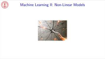
Quadratic predictors are nice but still a bit restricted: they can only go up and then down smoothly (or vice-vera). We can introduce another type of feature extractor that divides the input space into regions and allows the predicted value of each region tovary independently, This allows you to represent piecewise constant predictors (see figure). Specifically, each component of the feature vector corresponds to one region (e.g., [0, 1)) and is 1 if x lies in that region and 0 otherwise. Assuming the regions are disjoint, the weight associated with a component/region is exactly the predicted value. As you make the regions smaller, then you have more features, and the expressivity of your hypothesis class increases, allowing you to modelricher and richer functions. In the limit, you can essentially capture any predictor you want. This seems quite nice, but what is the catch? The drawback of these kinds of features is that you need alot of training data to learn thesepredictors. You need a sample within each interval to know its value, and there is no sharing of information across these intervals. Doing thistrick in d-dimensions rather than 1-dimension, your data requirements will go up exponentially in the dimension d!
Predictors with periodicity structureφ(x) [1, x, x2 , cos(3x)]Example: φ(2) [1, 2, 4, 0.96]43yf (x) [1, 1, 0.1, 1] · φ(x)2f (x) [3, 1, 0.1, 0.5] · φ(x)1F {fw (x) w · φ(x) : w R4 }0012345xJust throw in any features you wantCS22112
Quadratic and piecewise constant predictors are just two examples of an unboundedly large design space of possible feature extractors. Generally, the choice of features is informed by the prediction task that we wish to solve (either prior knowledge or preliminary data exploration). For example, if x represents time and we believe the true output y varies according to some periodic structure (e.g., traffic patterns repeatdaily, sales patterns repeat annually), then we might use periodic features such as cosine or sine to capture these trends. In this case, we can simply append the cosine of 3x to feature vector to represent such periodic functions at a particular frequency. Each feature might represent some type of structure in the data. If we have multiple types of structures, these can just be ”thrown in” intothe feature vector and let the learning algorithm decide what to use. Features represent what properties might be useful for prediction. If a feature is not useful, then the learning algorithm can (and hopefullywill) assign a weight close to zero to that feature. Of course, the more features one has, the harder learning becomes, and the more samplesyou will need.
Linear in what?Prediction:fw (x) w · φ(x)Linear in w?Linear in φ(x)?Linear in x?YesYesNo!Key idea: non-linearity Expressivity: score w · φ(x) can be a non-linear function of x Efficiency: score w · φ(x) always a linear function of wCS22114
Stepping back, how are we able to obtain non-linear predictors if we’re still using the machinery of linear predictors? This is perhaps a bitsurprising! You can think of this like pre-processing: the feature map φ is a way of transforming the inputs so that the function looks linearin this new space. Importantly, the score w · φ(x) is linear in the weights w and features φ(x). However, the score is not linear in x (it might not even makesense because x need not be a vector of numbers at all. In NLP, x is often a piece of text). Adding more features will generally make the prediction problem more linear, but this comes at the cost of learning and sample complexity.We have to learn more weights, one weight for each feature, which will require larger datasets The machinery of non-linear features combines the benefits of linear models, like simplicity and ease of optimization, with the benefits ofmore expressive models that capture nonlinear relations.
Linear classification3φ(x) [x1 , x2 ]f (x) sign([ 0.6, 0.6] · φ(x))2x210-1-2-3-3-2-10123x1Decision boundary is a lineCS22116
Now let’s turn from regression to classification. The story is pretty much the same: you can define arbitrary features to yield non-linear classifiers. Recall that in binary classification, the classifier (predictor) returns the sign of the score. The score is linear in the weights and the features, but the predictor is already not linear because of the sign operation. So, what do we meanby a classifier being non-linear or linear? Since it’s not helpful to talk about the linearity of f , we instead ask – can we make the classifier’s decision boundary non-linear? Last week, we only saw examples of classifiers with decision boundaries that are a straight line. Our goal now is to find classifiers that separatethe space of positives and negatives not by a line, but with a more complex boundary.
Quadratic classifiersφ(x) [x1 , x2 , x21 x22 ]f (x) sign([2, 2, 1] · φ(x))21x2Equivalently:(1if {(x 1 1)2 (x 2 1)2 2}f (x) 1 otherwise30-1-2-3-3-2-10123x1Decision boundary is a circleCS22118
Let us see how we can define a classifier with a non-linear decision boundary but still using the machinery of linear classifiers. Let’s try to construct a feature extractor that induces a decision boundary that is a circle: where everything inside is classified as 1 andeverything outside is classified as -1. As we saw before, we can add new features to get non-linear functions. In this case, we will add a new feature x21 x22 into the feature vector,and claim that a linear classifier with these features will give us a predictor with a circular decision boundary. If you group these terms, then you can rewrite the classifier to make it clear that it is the equation for the interior of a circle with radius 2. As a sanity check, we you can see that x [0, 0] results in a score of 0, which means that it is on the decision boundary. And as either of x1or x2 grow in magnitude (either x1 or x2 ), the contribution of the third feature dominates and the sign of the score will benegative. To recap, all we needed to do to get this decision boundary was to add these quadratic features into our linear classifier.
Visualization in feature spaceInput space: x [x1 , x2 ], decision boundary is a circleFeature space: φ(x) [x1 , x2 , x21 x22 ], decision boundary is a hyperplaneCS22120
Let’s try to understand the relationship between the non-linearity in x and linearity in φ(x). Click on the image to see the linked video (which is about polynomial kernels and SVMs, but the same principle applies here). In the input space x, the decision boundary which separates the red and blue points is a circle. We can also visualize the points in feature space, where each point is given an additional dimension x21 x22 . When we add a feature, we are essentially lifting the datapoints into a 3-dimensional space. In this three-dimensional feature space, a linear predictor (which is now defined by a hyperplane instead of a line) can in fact separate the redand blue points. This corresponds to the non-linear predictor in the original two-dimensional space, despite being a linear function in the lifted three dimensionalspace.
Summaryfw (x) w · φ(x)linear in w, φ(x)non-linear in x Regression: non-linear predictor, classification: non-linear decision boundary Types of non-linear features: quadratic, piecewise constant, etc.Non-linear predictors with linear machineryCS22122
To summarize, we have shown that the term ”linear” can be ambiguous: a predictor in regression can be non-linear in the input x but is sofar always linear with respect to the feature vector φ(x). The score is also linear with respect to the weights w, which is important for efficient learning. Classification is similar, except we talk about (non-)linearity of the decision boundary. We also saw many types of non-linear predictors that you could create by concocting various features (quadratic predictors, piecewise constantpredictors, periodic predictors). The takeaway is that linear models are surprisingly powerful! More sophisticated versions of this which are called kernel methods drove muchof the statistical machine learning gains in the early 2000s!
RoadmapTopics in the lecture:Nonlinear featuresFeature templatesNeural networksBackpropagationCS22124
Hopefully, you now have an idea of how to use linear models to learn non-linear predictors The main challenge though, is in defining these non-linear features. We will now cover feature templates, which is one way of defining flexible families of features
Feature extraction learningF {fw (x) sign(w · φ(x)) : w Rd }All predictorsFLearningFeature extractionfw Feature extraction: choose F based on domain knowledge Learning: choose fw F based on dataWant F to contain good predictors but not be too bigCS22126
Recall that the hypothesis class F is the set of predictors considered by the learning algorithm. In the case of linear predictors, the hypothesisclass F contains some function of w · φ(x) for all w (sign for classification, no sign for regression). This can be visualized as a set, shown inblue in this figure. Learning is the process of choosing a particular predictor fw from F given training data. But the question that we are currently concerned about is how do we choose F? We saw some options already: the set of linear predictors,the set of quadratic predictors which is a strict superset, etc., but what makes sense for a given application? If the hypothesis class doesn’t contain any good predictors, then no amount of learning can help. So the question when extracting features isreally whether they are powerful enough to express good predictors. It’s okay and expected that F will contain bad predictors as well, sincethe learning algorithm can avoid them. But we also don’t want F to be too big, or else learning becomes hard, not just computationally butalso statistically (which we’ll talk about more in the module on generalization). In essence, we want the smallest hypothesis class size that still contains good predictors.
Feature extraction with feature namesExample task:classifierstring (x)fw (x) sign(w · φ(x))valid email address? (y)Question: what properties of x might be relevant for predicting y?Feature extractor: Given x, produce set of (feature name, feature value) pairsabc@gmail.comxCS221 [features]feature extractor φarbitrary!length 10:1fracOfAlpha : 0.85contains @:1endsWith com : 1endsWith org : 0φ(x)28
To get some intuition about feature extraction, let us consider the task of predicting whether whether a string is a valid email address or not. We will assume the classifier fw is a linear classifier, which is given by some feature extractor φ. Feature extraction is a bit of an art that requires intuition about both the task and also what machine learning algorithms are capable of.The general principle is that features should represent properties of x which might be relevant for predicting y. Think about the feature extractor as producing a set of (feature name, feature value) pairs. For example, we might extract information aboutthe length, or fraction of alphanumeric characters, whether it contains various substrings, etc. It is okay to add features which turn out to be irrelevant, since the learning algorithm can always in principle choose to ignore the feature,though it might take more data to do so. We have been associating each feature with a name so that it’s easier for us (as humans) to interpret and develop the feature extractor. Thefeature names act like the analogue of comments in code. Mathematically, the feature name is not needed by the learning algorithm anderasing them does not change prediction or learning, but it is helpful for interpreting them within our overall system.
Prediction with feature namesWeight vector w RdFeature vector φ(x) Rdlength 10:-1.2fracOfAlpha :0.6contains @:3endsWith com:2.2endsWith org :1.4length 10:1fracOfAlpha :0.85contains @:1endsWith com:1endsWith org :0Score: weighted combination of featuresw · φ(x) Pdj 1wj φ(x)jExample: 1.2(1) 0.6(0.85) 3(1) 2.2(1) 1.4(0) 4.51CS22130
A feature vector formally is just a list of numbers, but we have endowed each feature in the feature vector with a name. The weight vector is also just a list of numbers, but we can give each weight the corresponding name as well. Since the score is simply the dot product between the weight vector and the feature vector. each feature weight wj determines how thecorresponding feature value φj (x) contributions to the prediction, and these contributions are aggregated in the score. If wj is positive, then the presence of feature j (φj (x) 1) favors a positive classification (e.g., ending with com). Conversely, if wj isnegative, then the presence of feature j favors a negative classification (e.g., length greater than 10). The magnitude of wj measures thestrength or importance of this contribution. Finally, keep in mind that these contributions are considered holistically. It might be tempting to think that a positive weight means that afeature is always positively correlated with the output. That is not necessarily true - the weights in a model work together, and a featurewith positive weight can even have negative correlation with the outcome. You may have seen an example of this in a stats course - calledsimpsons paradox - which you can look into if you find this intriguing.
Organization of features?abc@gmail.comxfeature extractor φarbitrary!length 10:1fracOfAlpha : 0.85contains @:1endsWith com : 1endsWith org : 0φ(x)Which features to include? Need an organizational principle.CS22132
How would we go about about creating good features? Here, we used our prior knowledge to define certain features (like whether an input contains @) which we believe are helpful for detectingemail addresses. But this is ad-hoc, and it’s easy to miss useful features (e.g. country codes in the ends with), and there might be other features which arepredictive but not intuitive. So, we need a more systematic way to go about constructing these features to try to capture all the features we might want.
Feature templatesDefinition: feature templateA feature template is a group of features all computed in a similar way.abc@gmail.comlast three characters a : 0aab : 0aac : 0com : 1zzz : 0Define types of pattern to look for, not particular patternsCS22134
A useful organization principle is a feature template, which groups all the features which are computed in a similar way. (People often usethe word ”feature” when they really actually mean ”feature template”.) Rather than defining individual features like endsWith com, we can define a single feature template that expands into all the features thatcomputes whether the input x matches any three characters. Typically, we will write a feature template as an English description with a blank ( ), which is to be filled in with an arbitrary value. The upshot is that we don’t need to know which particular patterns (e.g., three-character suffixes) are useful, but only that existence ofcertain patterns (e.g., three-character suffixes) are useful cue to look at. As long as this set can capture useful templates like .com, then thisfeature template will be useful It is then up to the learning algorithm to figure out which patterns are useful for predicting email addresses by assigning the appropriatefeature weights.
Feature templates example 1Input:abc@gmail.comFeature templateExample featureFraction of alphanumeric characters Fraction of alphanumeric characters : 0.85CS221Last three characters equalsLast three characters equals com: 1Length greater thanLength greater than 10: 136
Here are some other examples of feature templates. Note that an isolated feature (e.g., fraction of alphanumeric characters) can be treated as a trivial feature template with no blanks to befilled. In many cases, the feature value is binary (0 or 1) or within some discrete set (e.g. 1, ., 10), but they can also be real numbers.
Feature templates example 2Input:Latitude: 37.4068176Longitude: -122.1715122Feature templateExample feature namePixel intensity of image at rowLatitude is in [CS221,and column] and longitude is in [(,channel) Pixel intensity of image at row 10 and column 93 (red channel) : 0.8]Latitude is in [ 37.4, 37.5 ] and longitude is in [ -122.2, -122.1 ] : 138
As another example application, suppose the input is an aerial image along with the latitude/longitude corresponding to where the image wastaken. This type of input arises in poverty mapping and land cover classification. In this case, we might define one feature template corresponding to the pixel intensities at various pixel-wise row/column positions in theimage across all the 3 color channels (e.g., red, green, blue). Another feature template might define a family of binary features, one for each region of the world, where each region is defined by a boxover latitude and longitude. This is very similar to the piecewise constant predictors that we discussed earlier in the lecture, where we haveindicators for points that lie in a particular region.
Sparsity in feature vectorsabc@gmail.comlast character dsWithendsWitha :0b :0c :0d :0e :0f :0g :0h :0i :0j :0k :0l :0m:1n :0o :0p :0q :0r :0s :0t :0u :0v :0w :0x :0y :0z :0Compact representation:CS221{"endsWith m":1}40
In general, a feature template corresponds to many features, and sometimes, for a given input, most of the feature values are zero; that is,the feature vector is sparse. For example, in the email address prediction problem, we see that the vast number of endswith features are zeros for this address. In fact,only one of them can be one for this feature template. Of course, different feature vectors will have different non-zero features. But, in these cases, it is very inefficient to represent all the features explicitly, especially when you are using many different sparse featuretemplates. Instead, we can store only the values of the non-zero features, assuming all other feature values are zero by default. This compactrepresentation is shown at the bottom.
Two feature vector implementationsArrays (good for dense features):Dictionaries (good for sparse features):pixelIntensity(0,0) : 0.8pixelIntensity(0,1) : 0.6pixelIntensity(0,2) : 0.5pixelIntensity(1,0) : 0.5pixelIntensity(1,1) : 0.8pixelIntensity(1,2) : 0.7pixelIntensity(2,0) : 0.2pixelIntensity(2,1) : 0pixelIntensity(2,2) : 0.1fracOfAlpha : 0.85contains a : 0contains b : 0contains c : 0contains d : 0contains e : 0.contains @ : 1.[0.8, 0.6, 0.5, 0.5, 0.8, 0.7, 0.2, 0, 0.1]CS221{"fracOfAlpha":0.85, "contains @":1}42
In general, there are two common ways to implement feature vectors: using arrays (which are good for dense features) and using dictionaries(which are good for sparse features). Arrays assume a fixed ordering of the features and store the feature values as an array. This implementation is appropriate when the numberof nonzeros is significant (the features are dense). Pixel intensity is a good example, since there is a wide range of intensities and mostlocations have a non-zero pixel intensity. However, when we have sparsity, it is typically much more efficient to implement the feature vector as a dictionary (or a map) from stringsto doubles rather than a fixed-size array of doubles. The features not in the dictionary implicitly have a default value of zero. This sparseimplementation is useful for areas like natural language processing with linear predictors, and is what allows us to work efficiently over millionsof features and words because most of them never appear in an individual example. Dictionaries do incur extra overhead compared to arrays,and therefore dictionaries are much slower when the features are not sparse. One advantage of the sparse feature implementation is that you don’t have to instantiate all the set of possible features in advance; the weightvector can be initialized to empty {}, and only when a feature weight becomes non-zero do we store it. This means we can dynamicallyupdate a model with incrementally arriving data, which might instantiate new features.
SummaryF {fw (x) sign(w · φ(x)) : w Rd }Feature template:abc@gmail.comlast three characters a : 0aab : 0aac : 0com : 1zzz : 0Dictionary implementation:{"endsWith com":CS2211}44
The question we are concerned with in this section is how to define the hypothesis class F, which in the case of linear predictors is thequestion of what the feature extractor φ is. We saw earlier that the feature extractor can dramatically change the kinds of functions that we can reprensent. We showed how feature templates can be useful for organizing the definition of many features, and that we can use dictionaries to representsparse feature vectors efficiently. Stepping back, feature engineering is one of the most critical components in the practice of machine learning. It often does not get as muchattention as it deserves, mostly because it is a bit of an art and usually quite domain-specific. More powerful predictors such as neural networks will alleviate a lot of the burden of feature engineering (which is one of the reasons it isso popular), but even neural networks use feature vectors as the initial starting point, and therefore their effectiveness is still affected by thefeature representation.
RoadmapTopics in the lecture:Nonlinear featuresFeature templatesNeural networksBackpropagationCS22146
Now let’s dive into neural networks, first by understanding them as a model and hypothesis class.
Non-linear predictors4Linear predictors:fw (x) w · φ(x), φ(x) [1, x]y3210012345345345x43yNon-linear (quadratic) predictors:fw (x) w · φ(x), φ(x) [1, x, x2 ]210012x4Non-linear neural networks:fw (x) w · σ(Vφ(x)), φ(x) [1, x]y3210012xCS22148
Recall that our first hypothesis class was linear (in x) predictors, which for regression means that the predictors are lines. However, we also showed that you could get predictors that are non-linear in x by simply changing the feature extractor φ. For example,adding the feature x2 gave us quadratic predictors. One disadvantage of this approach is that if x were d-dimensional, one would need O(d2 ) features and corresponding weights to learn anarbitrary quadratic in d dimensions. This can present considerable computational and statistical challenges. We will show that neural networks are a way to build complex nonlinear predictors without creating a large number of complex featureextractors by hand What do neural networks get us? A common misconception that neural networks are more expressive than other models but this isnt necessarilytrue. You can define φ to be extremely large, to the point where it can approximate arbitrary smooth functions. This idea of using featuremaps to approximate complex functions is called a kernel based method. So, there is no inherent benefit in terms of expressive power to usingneural networks. Rather, one core benefit of neural networks is that they yield non-linear predictors in a more compact way and an often more computationallytractable way. For instance, you might not need O(d2 ) features to represent the desired non-linear predictor.
Motivating exampleExample: predicting car collisionInput: positions of two oncoming cars x [x1 , x2 ]Output: whether safe (y 1) or collide (y 1)Unknown: safe if cars sufficiently far: y sign( x1 x2 50
As a motivating example, consider the problem of predicting whether two cars are going to collide given the their positions (as measured fromdistance from one side of the road). In particular, let x1 be the position of one car and x2 be the position of the other car. Suppose the true output is 1 (safe) whenever the cars are separated by a distance of at least 1. This relationship can be represented by thedecision boundary which labels all points in the interior region between the two red lines as negative, and everything on the exterior (on eitherside) as positive. Of course, this true input-output relationship is unknown to the learning algorithm, which only sees training data. So, we want to learn thedecision boundary that separates the blue points from the yellow points. (This is essentially the famous XOR problem that was impossible tofit using linear classifiers. And you can see that no single line will separate these points.)
Decomposing the problem3h2 (x)21x2Test if car 1 is far right of car 2:h1 (x) 1[x1 x2 1]Test if car 2 is far right of car 1:h2 (x) 1[x2 x1 1]Safe if at least one is true:f (x) sign(h1 (x) h2 (x))0-1h1 (x)-2-3-3-2-10123x1CS221xh1 (x)h2 (x)f (x)[0, 2]01 1[2, 0]10 1[0, 0]00 1[2, 2]00 152
One way to motivate neural networks is the idea of problem decomposition. The intuition is to break up the full problem into two subproblems: the first subproblem tests if car 1 is to the far right of car 2; the secondsubproblem tests if car 2 is to the far right of car 1 Then the final output is 1 iff at least one of the two subproblems returns 1. Concretely, we can define h1
the feature vector and let the learning algorithm decide what to use. Features represent what properties might be useful for prediction. If a feature is not useful, then the learning algorithm can (and hopefully will) assign a weight close to zero to that feature. Of course, the more features one has, the harder learning becomes, and the more .