Transcription
LINEAR ALGEBRAGABRIEL NAGYMathematics Department,Michigan State University,East Lansing, MI, 48824.JULY 15, 2012Abstract. These are the lecture notes for the course MTH 415, Applied Linear Algebra,a one semester class taught in 2009-2012. These notes present a basic introduction tolinear algebra with emphasis on few applications. Chapter 1 introduces systems of linearequations, the Gauss-Jordan method to find solutions of these systems which transformsthe augmented matrix associated with a linear system into reduced echelon form, wherethe solutions of the linear system are simple to obtain. We end the Chapter with two applications of linear systems: First, to find approximate solutions to differential equationsusing the method of finite differences; second, to solve linear systems using floating-pointnumbers, as happens in a computer. Chapter 2 reviews matrix algebra, that is, we introduce the linear combination of matrices, the multiplication of appropriate matrices,and the inverse of a square matrix. We end the Chapter with the LU-factorization of amatrix. Chapter 3 reviews the determinant of a square matrix, the relation between anon-zero determinant and the existence of the inverse matrix, a formula for the inversematrix using the matrix of cofactors, and the Cramer rule for the formula of the solution of a linear system with an invertible matrix of coefficients. The advanced part ofthe course really starts in Chapter 4 with the definition of vector spaces, subspaces, thelinear dependence or independence of a set of vectors, bases and dimensions of vectorspaces. Both finite and infinite dimensional vector spaces are presented, however finitedimensional vector spaces are the main interest in this notes. Chapter 5 presents lineartransformations between vector spaces, the components of a linear transformation in abasis, and the formulas for the change of basis for both vector components and transformation components. Chapter 6 introduces a new structure on a vector space, called aninner product. The definition of an inner product is based on the properties of the dotproduct in Rn . We study the notion of orthogonal vectors, orthogonal projections, bestapproximations of a vector on a subspace, and the Gram-Schmidt orthonormalizationprocedure. The central application of these ideas is the method of least-squares to findapproximate solutions to inconsistent linear systems. One application is to find the bestpolynomial fit to a curve on a plane. Chapter 8 introduces the notion of a normed space,which is a vector space with a norm function which does not necessarily comes from aninner product. We study the main properties of the p-norms on Rn or Cn , which areuseful norms in functional analysis. We briefly discuss induced operator norms. The lastSection is an application of matrix norms. It discusses the condition number of a matrixand how to use this information to determine ill-conditioned linear systems. Finally,Chapter 9 introduces the notion of eigenvalue and eigenvector of a linear operator. Westudy diagonalizable operators, which are operators with diagonal matrix componentsin a basis of its eigenvectors. We also study functions of diagonalizable operators, withthe exponential function as a main example. We also discuss how to apply these ideasto find solution of linear systems of ordinary differential equations.Date: July 15, 2012,gnagy@math.msu.edu.
G. NAGY – LINEAR ALGEBRA July 15, 2012ITable of ContentsOverviewNotation and conventionsAcknowledgmentsChapter 5.5.Linear systemsRow and column picturesRow pictureColumn pictureExercisesGauss-Jordan methodThe augmented matrixGauss elimination operationsSquare systemsExercisesEchelon formsEchelon and reduced echelon formsThe rank of a matrixInconsistent linear systemsExercisesNon-homogeneous equationsMatrix-vector productLinearity of matrix-vector productHomogeneous linear systemsThe span of vector setsNon-homogeneous linear systemsExercisesFloating-point numbersMain definitionsThe rounding functionSolving linear systemsReducing rounding errorsExercisesChapter 2.Matrix algebra2.1. Linear transformations2.1.1. A matrix is a function2.1.2. A matrix is a linear function2.1.3. Exercises2.2. Linear combinations2.2.1. Linear combination of matrices2.2.2. The transpose, adjoint, and trace of a matrix2.2.3. Linear transformations on matrices2.2.4. Exercises2.3. Matrix multiplication2.3.1. Algebraic definition2.3.2. Matrix composition2.3.3. Main properties2.3.4. Block 8303134353537384042434343475051515255565757596162
IIG. NAGY – LINEAR ALGEBRA july 15, 20122.3.5. Matrix commutators2.3.6. Exercises2.4. Inverse matrix2.4.1. Main definition2.4.2. Properties of invertible matrices2.4.3. Computing the inverse matrix2.4.4. Exercises2.5. Null and range spaces2.5.1. Definition of the spaces2.5.2. Main properties2.5.3. Gauss operations2.5.4. Exercises2.6. LU-factorization2.6.1. Main definitions2.6.2. A sufficient condition2.6.3. Solving linear systems2.6.4. ExercisesChapter 3.1. Definitions and properties3.1.1. Determinant of 2 2 matrices3.1.2. Determinant of 3 3 matrices3.1.3. Determinant of n n matrices3.1.4. Exercises3.2. Applications3.2.1. Inverse matrix formula3.2.2. Cramer’s rule3.2.3. Determinants and Gauss operations3.2.4. Exercises91919598101102102104105107Chapter 1.Vector spacesSpaces and subspacesSubspacesThe span of finite setsAlgebra of subspacesInternal direct sumsExercisesLinear dependenceLinearly dependent setsMain propertiesExercisesBases and dimensionBasis of a vector spaceDimension of a vector spaceExtension of a set to a basisThe dimension of subspace additionExercisesVector componentsOrdered 128130131131
G. NAGY – LINEAR ALGEBRA July 15, 20124.4.2.4.4.3.Vector components in a basisExercisesChapter near transformations137Linear transformationsThe null and range spacesInjections, surjections and bijectionsNullity-Rank TheoremExercisesProperties of linear transformationsThe inverse transformationThe vector space of linear transformationsLinear functionals and the dual spaceExercisesThe algebra of linear operatorsPolynomial functions of linear operatorsFunctions of linear operatorsThe commutator of linear operatorsExercisesTransformation componentsThe matrix of a linear transformationAction as matrix-vector productComposition and matrix productExercisesChange of basisVector componentsTransformation componentsDeterminant and trace of linear 4156157158159160160162165167168168170173175Chapter 3.IIIInner product spacesDot productDot product in R2Dot product in FnExercisesInner productInner productInner product normNorm distanceExercisesOrthogonal vectorsDefinition and examplesOrthonormal basisVector componentsExercisesOrthogonal projectionsOrthogonal projection onto subspacesOrthogonal 92192194196198199199202205
IVG. NAGY – LINEAR ALGEBRA july 15, 20126.5. Gram-Schmidt method6.5.1. Exercises6.6. The adjoint operator6.6.1. The Riesz Representation Theorem6.6.2. The adjoint operator6.6.3. Normal operators6.6.4. Bilinear forms6.6.5. ExercisesChapter 2.7.4.3.7.4.4.Approximation methodsBest approximationFourier expansionsNull and range spaces of a matrixExercisesLeast squaresThe normal equationLeast squares fitLinear correlationQR-factorizationExercisesFinite difference methodDifferential equationsDifference quotientsMethod of finite differencesExercisesFinite element methodDifferential equationsThe Galerkin methodFinite element methodExercisesChapter 8.Normed spaces8.1. The p-norm8.1.1. Not every norm is an inner product norm8.1.2. Equivalent norms8.1.3. Exercises8.2. Operator norms8.2.1. Exercises8.3. Condition numbers8.3.1. ExercisesChapter 2255256262263265Spectral decomposition2669.1. Eigenvalues and eigenvectors9.1.1. Main definitions9.1.2. Characteristic polynomial9.1.3. Eigenvalue multiplicities9.1.4. Operators with distinct eigenvalues9.1.5. Exercises9.2. Diagonalizable operators266266269270272274275
G. NAGY – LINEAR ALGEBRA July 15, 20129.2.1. Eigenvectors and diagonalization9.2.2. Functions of diagonalizable operators9.2.3. The exponential of diagonalizable operators9.2.4. Exercises9.3. Differential equations9.3.1. Non-repeated real eigenvalues9.3.2. Non-repeated complex eigenvalues9.3.3. Exercises9.4. Normal operators9.4.1. ExercisesChapter 10.Appendix10.1. Review exercises10.2. Practice Exams10.3. Answers to exercises10.4. Solutions to Practice 01310317336356
G. NAGY – LINEAR ALGEBRA July 15, 20121OverviewLinear algebra is a collection of ideas involving algebraic systems of linear equations,vectors and vector spaces, and linear transformations between vector spaces.Algebraic equations are called a system when there is more than one equation, and theyare called linear when the unknown appears as a multiplicative factor with power zero or one.An example of a linear system of two equations in two unknowns is given in Eqs. (1.3)-(1.4)below. Systems of linear equations are the main subject of Chapter 1.Examples of vectors are oriented segments on a line, plane, or space. An oriented segmentis an ordered pair of points in these sets. Such ordered pair can be drawn as an arrow thatstarts on the first point and ends on the second point. Fix a preferred point in the line, planeor space, called the origin point, and then there exists a one-to-one correspondence betweenpoints in these sets and arrows that start at the origin point. The set of oriented segmentswith common origin in a line, plane, and space are called R, R2 and R3 , respectively.A sketch of vectors in these sets can be seen in Fig. 1. Two operations are defined onoriented segments with common origin point: An oriented segment can be stretched orcompressed; and two oriented segments with the same origin point can be added using theparallelogram law. An addition of several stretched or compressed vectors is called a linearcombination. The set of all oriented segments with common origin point together with thisoperation of linear combination is the essential structure called vector space. The origin ofthe word “space” in the term “vector space” originates precisely in these examples, whichwere associated with the physical space.000Figure 1. Example of vectors in the line, plane, and space, respectively.Linear transformations are a particular type of functions between vector spaces thatpreserve the operation of linear combination. An example of a linear transformation is a2 2 matrix A 13 24 together with a matrix-vector product that specifies how this matrixtransforms a vector on the plane into another vector on the plane. The result is thus afunction A : R2 R2 .These notes try to be an elementary introduction to linear algebra with few applications.Notation and conventions. We use the notation F {R, C} to mean that F R orF C. Vectors will be denoted by boldface letters, like u and v. The exception are acolumn vectors in Fn which are denoted in sanserif, like u and v. This notation permitsto differentiate between a vector and its components on a basis. In a similar way, lineartransformations between vector spaces are denoted by boldface capital letters, like T andS. The exception are matrices in Fm,n which are denoted by capital sanserif letters like Aand B. Again, this notation is useful to differentiate between a linear transformation and its
2G. NAGY – LINEAR ALGEBRA july 15, 2012components on two bases. Below is a list of few mathematical symbols used in these notes:R Set of real numbers,Q Set of rational numbers,Z Set of integer numbers,N Set of positive integers,{0}Zero set, Union of sets,: Definition, For all,ProofBeginning of a proof,Example Beginning of an example, Empty set, Intersection of sets, Implies,There exists, End of a proof,CEnd of an example.Acknowledgments. I thanks all my students for pointing out several misprints and forhelping make these notes more readable. I am specially grateful to Zhuo Wang and WenningFeng.
G. NAGY – LINEAR ALGEBRA July 15, 20123Chapter 1. Linear systems1.1. Row and column pictures1.1.1. Row picture. A central problem in linear algebra is to find solutions of a system oflinear equations. A 2 2 linear system consists of two linear equations in two unknowns.More precisely, given the real numbers A11 , A12 , A21 , A22 , b1 , and b2 , find all numbers xand y solutions of both equationsA11 x A12 y b1 ,(1.1)A21 x A22 y b2 .(1.2)These equations are called a system because there is more than one equation, and they arecalled linear because the unknowns, x and y, appear as multiplicative factors with powerzero or one (for example, there is no term proportional to x2 or to y 3 ). The row picture ofa linear system is the method of finding solutions to this system as the intersection of allsolutions to every single equation in the system. The individual equations are called rowequations, or simply rows of the system.Example 1.1.1: Find all the numbers x and y solutions of the 2 2 linear system2x y 0,(1.3) x 2y 3.(1.4)Solution: The solution to each row of the system above is found geometrically in Fig. 2.ysecond row2y x 3first rowy 2x2(1,2)1 3xFigure 2. The solution of a 2 2 linear system in the row picture is theintersection of the two lines, which are the solutions of each row equation.Analytically, the solution can be found by substitution:2x y 0 y 2x x 4x 3½ x 1,y 2.CAn interesting property of the solutions to any 2 2 linear system is simple to proveusing the row picture, and it is the following result.Theorem 1.1.1. Given any 2 2 linear system, only one of the following statements holds:(i) There exists a unique solution;(ii) There exist infinitely many solutions;(iii) There exists no solution.
4G. NAGY – LINEAR ALGEBRA july 15, 2012It is interesting to remark what cannot happen, for example there is no 2 2 linear systemhaving only two solutions. Unlike the quadratic equation x2 5x 6 0, which has twosolutions given by x 2 and x 3, a 2 2 linear system has only one solution, or infinitelymany solutions, or no solution at all. Examples of these three cases, respectively, are givenin Fig. 3.yyyxxxFigure 3. An example of the cases given in Theorem 1.1.1, cases (i)-(iii).Proof of Theorem 1.1.1: The solutions of each equation in a 2 2 linear system representsa line in R2 . Two lines in R2 can intersect at a point, or can be coincident, or can be parallelbut not coincident. These are the cases given in (i)-(iii). This establishes the Theorem. We now generalize the definition of a 2 2 linear system given in the Example 1.1.1 tom equations of n unknowns.Definition 1.1.2. An m n linear system is a set of m 1 linear equations in n 1unknowns is the following: Given the coefficients numbers Aij and the source numbers bi ,with i 1, · · · , m and j 1, · · · n, find the real numbers xj solutions ofA11 x1 · · · A1n xn b1.Am1 x1 · · · Amn xn bm .Furthermore, an m n linear system is called consistent iff it has a solution, and it iscalled inconsistent iff it has no solutions.Example 1.1.2: Find all numbers x1 , x2 and x3 solutions of the 2 3 linear systemx1 2x2 x3 1(1.5) 3x1 x2 8x3 2Solution: Compute x1 from the first equation, x1 1 2x2 x3 , and substitute it in thesecond equation, 3 (1 2x2 x3 ) x2 8x3 2 5x2 5x3 5 x2 1 x3 .Substitute the expression for x2 in the equation above for x1 , and we obtainx1 1 2 (1 x3 ) x3 1 2 2x3 x3 x1 1 3x3 .Since there is no condition on x3 , the system above has infinitely many solutions parametrized by the number x3 . We conclude that x1 1 3x3 , and x2 1 x3 , while x3 is free.CExample 1.1.3: Find all numbers x1 , x2 and x3 solutions of the 3 3 linear system2x1 x2 x3 2 x1 2x2 1x1 x2 2x3 2.(1.6)
G. NAGY – LINEAR ALGEBRA July 15, 20125Solution: While the row picture is appropriate to solve small systems of linear equations,it becomes difficult to carry out on 3 3 and bigger linear systems. The solution x1 , x2 , x3of the system above can be found as follows: Substitute the second equation into the first,x1 1 2x2 x3 2 2x1 x2 2 2 4x2 x2 x3 4 5x2 ;then, substitute the second equation and x3 4 5x2 into the third equation,( 1 2x2 ) x2 2(4 5x2 ) 2 x2 1,and then, substituting backwards, x1 1 and x3 1. We conclude that the solution is asingle point in space given by (1, 1, 1).CThe solution of each separate equation in the examples above represents a plane in R3 . Asolution to the whole system is a point that belongs to the three planes. In the 3 3 systemin Example 1.1.3 above there is a unique solution, the point (1, 1, 1), which means that thethree planes intersect at a single point. In the general case, a 3 3 system can have a uniquesolution, infinitely many solutions or no solutions at all, depending on how the three planesin space intersect among them. The case with unique solution was represented in Fig. 4,while two possible situations corresponding to no solution are given in Fig. 5. Finally, twocases of 3 3 linear system having infinitely many solutions are pictured in Fig 6, where inthe first case the solutions form a line, and in the second case the solutions form a planebecause the three planes coincide.Figure 4. Planes representing the solutions of each row equation in a 3 3linear system having a unique solution.Figure 5. Two cases of planes representing the solutions of each row equation in 3 3 linear systems having no solutions.Solutions of linear systems with more than three unknowns can not be represented in thethree dimensional space. Besides, the substitution method becomes more involved to solve.As a consequence, alternative ideas are needed to solve such systems. We now discuss one
6G. NAGY – LINEAR ALGEBRA july 15, 2012Figure 6. Two cases of planes representing the solutions of each row equation in 3 3 linear systems having infinitely many solutions.of such ideas, the use of vectors to interpret and find solutions of linear systems. In the nextSection we introduce another idea, the use of matrices and vectors to solve linear systemsfollowing the Gauss-Jordan method. This latter procedure is suitable to solve large systemsof linear equations in an efficient way.1.1.2. Column picture. Consider again the linear system in Eqs. (1.3)-(1.4) and introducea change in the names of the unknowns, calling them x1 and x2 instead of x and y. Theproblem is to find the numbers x1 , and x2 solutions of2x1 x2 0,(1.7) x1 2x2 3.(1.8)We know that the answer is x1 1, x2 2. The row picture consisted in solving each rowseparately. The main idea in the column picture is to interpret the 2 2 linear system asan addition of new objects, column vectors, in the following way,· · · 0 12.(1.9)x2 x1 32 1The new objects are called column vectors and they are denoted as follows,· · · 2 10A1 , A2 , b . 123We can represent these vectors in the plane, as it is shown in Fig. 7.x23bA222 1x1 1A1Figure 7. Graphical representation of column vectors in the plane.The column vector interpretation of a 2 2 linear system determines an addition lawof vectors and a multiplication law of a vector by a number. In the example above, we
G. NAGY – LINEAR ALGEBRA July 15, 20127know that the solution is given by x1 1 and x2 2, therefore in the column pictureinterpretation the following equation must hold· · · 2 10 2 . 123The study of this example suggests that the multiplication law of a vector by numbers andthe addition law of two vectors can be defined by the following equations, respectively,· · · · · 1( 1)22 22 22 , .2(2)2 14 1 4The study of several examples of 2 2 linear systems in the column picture determines thefollowing definition.· · uvDefinition 1.1.3. The linear combination of the 2-vectors u 1 and v 1 , withu2v2the real numbers a and b, is defined as follows,· · · uvau1 bv1a 1 b 1 .u2v2au2 bv2A linear combination includes the particular cases of addition (a b 1), and multiplication of a vector by a number (b 0), respectively given by,· · · · · u1v1u1 v1u1au1 ,a .u2v2u2 v2u2au2The addition law in terms of components is represented graphically by the parallelogramlaw, as it can be seen in Fig. 8. The multiplication of a vector by a number a affects thelength and direction of the vector. The product au stretches the vector u when a 1 andit compresses u when 0 a 1. If a 0 then it reverses the direction of u and it stretcheswhen a 1 and compresses when 1 a 0. Fig. 8 represents some of these possibilities.Notice that the difference of two vectors is a particular case of the parallelogram law, as itcan be seen in Fig. 9.x2v2V WaVVa 1 V(v w)Va 12aVWw2w1v1(v w)0 a 1x11Figure 8. The addition of vectors can be computed with the parallelogramlaw. The multiplication of a vector by a number stretches or compressesthe vector, and changes it direction in the case that the number is negative.The column picture interpretation of a general 2 2 linear system given in Eqs. (1.1)-(1.2)is the following: Introduce the coefficient and source column vectors· · · A11A12bA1 , A2 , b 1 ,(1.10)A21A22b2
8G. NAGY – LINEAR ALGEBRA july 15, 2012V WV WV ( W)VVW WWFigure 9. The difference of two vectors is a particular case of the parallelogram law of addition of vectors.and then find the coefficients x1 and x2 that change the length of the coefficient columnvectors A1 and A2 such that they add up to the source column vector b, that is,A1 x1 A2 x2 b.For example, the column picture of the linear system in Eqs. (1.7)-(1.8) is given in Eq. (1.9).The solution of this system are the numbers x1 1 and x2 2, and this solution isrepresented in Fig. 10.x2x2442 A22 A2b2A2 22 1Ax1 2 1x11Figure 10. Representation of the solution of a 2 2 linear system in thecolumn picture.The existence and uniqueness of solutions in the case of 2 2 systems can be studiedgeometrically in the column picture as it was done in the row picture. In the latter case wehave seen that all possible 2 2 systems fall into one of these three cases, unique solution,infinitely many solutions and no solutions at all. The proof was to study all possible waystwo lines can intersect on the plane. The same existence and uniqueness statement canbe proved in the column picture. In Fig. 11 we present these three cases in both row andcolumn pictures. In the latter case the proof is to study all possible relative positions of thecolumn vectors A1 , A2 , and b on the plane.We see in Fig. 11 that the first case corresponds to a system with unique solution. Thereis only one linear combination of the coefficient vectors A1 and A2 which adds up to b. Thereason is that the coefficient vectors are not proportional to each other. The second casecorresponds to the case of infinitely many solutions. The coefficient vectors are proportionalto each other and the source vector b is also proportional to them. So, there are infinitelymany linear combinations of the coefficient vectors that add up to the source vector. The lastcase corresponds to the case of no solutions. While the coefficient vectors are proportional toeach other, the source vector is not proportional to them. So, there is no linear combinationof the coefficient vectors that add up to the source vector.
G. NAGY – LINEAR ALGEBRA July 15, 2012yy9yxxx2xx2x2bA2bA1A2bA1A1x1A2x1x1Figure 11. Examples of a solutions of general 2 2 linear systems havinga unique, infinitely many, and no solution, represented in the row pictureand in the column picture.The ideas in the column picture can be generalized to m n linear equations, which givesrise to the generalization to m-vectors of the definitions of linear combination presentedabove. u1v1 . . Definition 1.1.4. The linear combination of the m-vectors u . and v . umvmwith the real numbers a, b is defined as follows u1v1au1 bv1 .a . b . .umvmaum bvmThis definition can be generalized to an arbitrary number of vectors. Column vectorsprovide a new way to denote an m n system of linear equations.Definition 1.1.5. An m n linear system of m 1 linear equations in n 1 unknownsis the following: Given the coefficient m-vectors A1 , · · · , An and the source m-vector b, findthe real numbers x1 , · · · , xn solution of the linear combinationA1 x1 · · · An xn b.For example, recall the 3 3 system given as the second system in Eq. (1.6). This systemin the column picture is the following: Find numbers x1 , x2 and x3 such that 2112 1 x1 2 x2 0 x3 1 .(1.11)1 12 2These are the main ideas in the column picture. We will see later that linear algebraemerges from the column picture. In the next Section we introduce the Gauss-Jordanmethod, which is a procedure to solve large systems of linear equations in an efficient way.Further reading. For more details on the row picture see Section 1.1 in Lay’s book [2].There is a clear explanation of the column picture in Section 1.3 in Lay’s book [2]. See alsoSection 1.2 in Strang’s book [4] for a shorter summary of both the row and column pictures.
10G. NAGY – LINEAR ALGEBRA july 15, 20121.1.3. Exercises.1.1.1.- Use the substitution method to findthe solutions to the 2 2 linear system2x y 1,x y 5.1.1.2.- Sketch the three lines solution ofeach row in the systemx 2y 2x y 2y 1.Is this linear system consistent?1.1.3.- Sketch a graph representing the solutions of each row in the following nonlinear system, and decide whether ithas solutions or not,x2 y 2 4x y 0.1.1.4.- Graph on the plane the solution ofeach individual equation of the 3 2 linear system system3x y 0,x 2y 4, x y 2,and determine whether the system isconsistent or inconsistent.1.1.5.- Show that the 3 3 linear systemx y z 2,x 2y 3z 1,y 2z 0,is inconsistent, by finding a combinationof the three equations that ads up to theequation 0 1.1.1.6.- Find all values of the constant ksuch that there exists infinitely manysolutions to the 2 2 linear systemkx 2y 0,x ky 0.21.1.7.- Sketch a graph of the vectors» –» –» –121A1 , A2 , b .21 1Is the linear system A1 x1 A2 x2 bconsistent? If the answer is “yes,” findthe solution.1.1.8.- Consider the vectors» –» –4 2A1 , A2 ,2 1b » –2.0(a) Graph the vectors A1 , A2 and b onthe plane.(b) Is the linear system A1 x1 A2 x2 bconsistent?» –6(c) Given the vector c , is the3linear system A1 x1 A2 x2 c consistent? If the answer is “yes,” isthe solution unique?1.1.9.- Consider the vectors» –» – 24,, A2 A1 12ˆ and given a real number h, set c h2 .Find all values of h such that the systemA1 x1 A2 x2 c is consistent.1.1.10.- Show that the three vectors belowlie on the same plane, by expressing thethird vector as a linear combination ofthe first two, where2 32 32 3111A1 415 , A2 425 , A3 435 .201Is the linear systemA1 x1 A2 x2 A3 x3 0consistent? If the answer is “yes,” is thesolution unique?
G. NAGY – LINEAR ALGEBRA July 15, 2012111.2. Gauss-Jordan method1.2.1. The augmented matrix. Solutions to m n linear systems can be obtained inan efficient way using the Gauss-Jordan method. Efficient here means to perform as fewalgebraic operations as possible either to find the solution or to show that the solution doesnot exist. Before introducing this method, we need several definitions.Definition 1.2.1. The coefficients matrix, the source vector, and the augmentedmatrix of the m n linear systemA11 x1 · · · A1n xn b1.Am1 x1 · · · Amn xn bm ,are given by, respectively, A11 A .Am1······ A1n. ,. Amn b1 b . ,bm A11 A b . Am1···A1n.···Amn b1 . . bmWe call A an m n matrix, with m the number of rows and n the number of columns.The source vector b is a particular case of an m 1 matrix. The augmented matrix of anm n linear system is given by the coefficient matrix and the source vector together, henceit is an m (n 1) matrix.Example 1.2.1: Find the coefficient matrix, the source vector and the augmented matrixof the 2 2 linear system2x1 x2 0,(1.12) x1 2x2 3.(1.13)Solution: The coefficient matrix is 2 2, the source vector is 2 1, and the augmentedmatrix is 2 3, given respectively by · · · 2 102 1 0A , b , [A b] (1.14). 123 12 3CExample 1.2.2: Find the coefficient matrix, the source vector and the augmented matrixof the 2 3 linear system2x1 x2 0, x1 2x2 3x3 0.Solution: The coefficient matrix is 2 3, the source vector is 2 1,matrix is 2 4, given respectively by· · ·2 1 002 10A , b , [A b] 12 30 123and the augmented 0.0Notice that the coefficent matrix in this example is equal to the augmented matrix in theprevious Example. This means that the vertical separator in the definition of the augmented
12G. NAGY – LINEAR ALGEBRA july 15, 2012matrix is important. If on
Matrix algebra 43 2.1. Linear transformations 43 2.1.1. A matrix is a function 43 2.1.2. A matrix is a linear function 47 2.1.3. Exercises 50 2.2. Linear combinations 51 2.2.1. Linear combination of matrices 51 2.2.2. The transpose, adjoint, and trace of a matrix 52 2.2.3. Linear transformations on matrices 55