Transcription
An Introduction to GISUsing QGIS (v. 3.0)Author: Michael L. Tregliamtreglia@gmail.com13 May 2018License: This work is licensed under a Creative Commons AttributionNonCommercial-ShareAlike 4.0 International License. Please see the following websitefor complete license details or contact Michael Treglia at mtreglia@gmail.com withconcerns. egalcode
Opening NotesOpen-source tools for various types of work, are constantly expanding. Herein, Iprovide a tutorial of QGIS (www.qgis.org), which is capable of almost any GIS operationI’ve ever needed, either on its own, or using the various plugins and associated tools.QGIS installs and directly links with other programs including SAGA GIS and GRASSGIS, allowing users to take advantage of cooperation among the free and open sourcesoftware developers. Furthermore, data can be exported to a variety of formats, for usein other programs.My goal here is to provide a basic skill-set to the new GIS/QGIS user, so they maynavigate the software for their own work, and further explore its capabilities. Thistutorial is by no-means comprehensive. I suggest users browse and search the QGISdocumentation (https://qgis.org/en/docs/index.html) when they are stuck, or make useof relevant support channels urthermore, a lot of examples are given here without going into intricacies of analysis.Thus, I suggest before quantitative analytics, users read further on the tools/analysesthat can be employed.1
Table of ContentsOpening Notes . 1Table of Contents. 2Installing QGIS . 4Installing Plugins . 5Data Sources Used in this Tutorial . 6Get to Know QGIS . 7Opening Files (General) . 8Open Shapefiles, . 8Open Delimited Text Layer (e.g., points based on a table with Coordinates) . 9Add a Background Layer . 12Open and Manipulate a Raster Layer . 12Projections . 15Projection of Layers and Project . 15Changing Projections (CRS) . 16Changing Project CRS. 16Changing Vector CRS (for a Shapefile or Text-Delimited Layer) .17Changing Raster CRS . 18Geo-Processing of Data Layers and Associated Tables . 20Some Basic Vector Operations . 20Clipping (Remove unwanted sections of a layer, based on bounds of anotherLayer) . 20Difference Clip (Clip out the inner area of a polygon) . 22View and Edit the Attribute Table . 232
Spatial Join . 24Some Basic Raster Operations . 26Calculate Slope from a DEM . 26Reclassify Raster . 28Raster Calculator . 32Using Vector and Raster Datasets Together . 34Clipping a Raster . 34Compute Zonal Statistics for Polygons . 36Making a Quality Map . 37Setting up for a Map . 37Putting Everything Together . 40Adding the Map of interest to the Layout . 40Adding Gridlines and Coordinates . 40Adding Scale Bar, North Arrow, and Legend . 42Adding an Inset . 44Final Formatting and Exporting the Map. 45Exporting the Map . 45Closing Remarks. 473
Installing QGISI generally recommend working with the most recent version of QGIS available, with themost recent features, or the most recent Long Term Release, which is designed to bemaintained with bug-fixes and such for the next three release cycles. Long term releasesmight not have the most newest features found in the most recent version, but focus isbroader stability across time. At the time of writing, the most recent version is 3.0.2; thelong-term release is 2.18.9. Everything presented herein was tested using QGIS 3.0.2, 64bit, on Windows 10. Though there have been some changes since 2.18.x, the generalworkflows will be consistent. (Releases are denoted as x.y.z, where changes in ‘x’ denotessome potentially larger changes in the software, changes in ‘y’ denote additions offeatures and bug fixes, and changes in ‘z’ generally reflect bug-fixes.)For Windows users:Download and run the standalone installer, available ml (QGIS Standalone Installer Version3.0.2 will be sufficient; the OSGeo4W installer gives more advanced options, but is notneeded). When it gives you the option, you do not need to download the sample datasets,although feel free to and use them for other tutorials or examples.For Mac OS users:Download files should be available on the main QGIS download page. (At time ofwriting, when clicking to expand the box for “MacOS” from a non-Mac computer, the4
page scrolls to the bottom; if this happens, users should scroll up to find the downloadlinks!)For Linux Users:Follow instructions provided s.html#linux.Installing PluginsOne of the strengths of QGIS is the availability of capable plugins that have been writtenfor it. To see what plugins are installed, open QGIS by double-clicking on the “QGISDesktop” icon on your desktop or in your start menu. Then, click the Plugins menu at the top of the main QGIS window, and navigateto “Manage and Install Plugins”. When the Plugins window opens, search for the following plugins and installthem if they are not indicated as already installed (having a checked- orunchecked-box to the left of the name; uninstalled plugins will have a puzzlepiece emblem next to the name):o QuickMapServiceso Processing (installed by default) To ensure these plugins are active, make sure the box next to the name has acheck-mark in it.5
Data Sources Used in this TutorialThe data sources used in this tutorial are available for download in a single .zip folder, atthe URL where you accessed this document. Individual data layers and original sourcesare listed below. Please see the URLs for the original sources or the included metadatafor individual layers for more detail. Throughout the document, I primarily refer tolayers with the italicized names given below.Text Delimited Table Copperhead Data – “Brazos County A contortrix TxCentral.csv” – Specimenlocations for copperheads, Agkistrodon contortrix, in Brazos County, Texas,provided by the Biodiversity Research and Teaching Collections at Texas A&MUniversity (https://brtc.tamu.edu/). Most localities were definitely collected inthe WGS84 datum; the others are assumed to be for this tutorial.Vector Data (Shapefiles)The following layers for Brazos County and the city of College Station, TX were accessedfrom the City of College Station GIS Department in 2014 (newer files may be availableat: http://www.cstx.gov/index.aspx?page 3683).1) County Boundary – Brazos County Boundary 8-20-02.shp (in/CountyBoundary)2) City Limits – City Limits.shp (in /CityBoundary)3) Rivers and Streams – Rivers and Streams.shp (in: /RiversStreams”)6
Raster DataThe raster dataset used in this tutorial is the 1 Arc-second ( 30m) Digital ElevationModel from the U.S. Geological Survey DEM – imgn31w097 1.img (in /DEM 1ArcSec)Get to Know QGISOpen QGIS on your computer using the QGIS Desktop icon in your Start Menu orDesktop. By default, only one pane is likely open – the “Layers/Browser” pane on the leftside. You can adjust what is open by going to the “View” menu from the toolbar,and mouse-over “Panels”, and see different options. Explore icons by hovering over them with the mouse; click on menu-bar items toexplore the drop-down menus. To save the project click the “Save” icon and designate a file location. When youre-open a project, any layers that you were using should be in the samelocations on your computer; if they are not, you will need to re-designate theappropriate file paths. If you transfer data and a project file to anothercomputer, keep the files in the same locations relative to one another and theproject should open without a problem. Make sure to periodically save theproject as you work. In the latest versions, QGIS automatically shows the mostrecent projects. You can simply click a desired project to return to it, or otherwisenavigate through QGIS to proceed with a new project.7
Opening Files (General)Starting with version 3.0.0, QGIS has a universal Data Source Manager that facilitatesopening myriad types of files from a central interface. The icon, pictured at left, shouldbe the top-most on the left side of the screen. Users can also access it via “CTRL L” (onWindows) or going to “Layer” on the toolbar at the top and finding it. As with earlierversions of QGIS, users can still go to “Layer” - [Desired Layer Type] to load specifictypes of data, and this will call the Data Source Manager with the appropriate tab.Many common spatial data formats can also be opened by going to the “Browser” pane,navigating to the file location, and clicking/dragging the file into the general view or intothe “Layers” pane.Open Shapefiles,Shapefiles (.shp extension) are one file format of vector data (points/lines/polygons)commonly used in GIS. Though these are largely replaced by files within ESRI FileGeodatabases (.gdb extension) in ESRI products and Geopackage (.gpkg extension) inQGIS, a lot of datasets are still distributed as shapefiles. Within the Data Source Manager, click the “Vector” tab on the left (Or use“Layer” menu from the toolbar and navigate to “Add Layer” - “Add VectorLayer”)o Set the Source Type to “File” and Encoding to “System”.o Click “Browse” and navigate to the appropriate files, using the appropriatefile types (for Shapefiles, set to “ESRI Shapefiles [OGR] (*.shp)”).8
o Select County Boundary, City Limits, and Rivers and Stream layersrespectively, and click the “Add” button.**Note –To access data from ESRI Geodatabase (.gdb files; not used inthis exercise), set “Source Type” to “Directory”, and navigate to .gdb files. Adjust the layer order by clicking and dragging layers up and down in the“Layers” pane.o Put Rivers and Streams on top, then City Limits, and County Boundary To adjust layer symbology (how the data appear):o Right click on individual layers and select “Properties” (or Double Click onthe layer)o Select “Style” on the left; click on a symbol in the “Symbol Layers” box,and customize to your liking. You can also open a “Layer Styling” panel via “View” on thetoolbar - “Panels” - “Layer Styling” To view the tabular data associated with a layer, right click on the layer and select“Open Attribute Table”. To view information about a layer at a specific point in space, click on the“Identify Features” icon on the tool bar, and click on the point of interest. Thedefault setting show information about the layer highlighted in the “Layers” pane.Open Delimited Text Layer (e.g., points based on a table with Coordinates) In the Data Source Manager “Add Delimited Text Layer” icon. (See exampledialogue box on next page.)9
o Navigate to the appropriate file (Copperhead Data; “Brazos County Acontortrix.csv”)o Expand the “File Format” section and select the appropriate text delimiter(comma for this file).o Expand the “Records and Fields” section – if the first line contains fieldnames (column names) as in this case, make sure the “First record hasfield names” box is checked.o Expand the “Geometry Definition” section (typically “Point Coordinates”),and identify fields for X and Y coordinates (e.g., Longitude and Latitude,respectively).o If the data are based on a geographic projection Decimal Degrees areexpected as with the Copperhead data; if data are as Degrees MinutesSeconds, check the “DMS Coordinates” box. By default, the CRS (Coordinate Reference System) for the newlayer is set to the CRS of the project, Lat/Long, WGS84 (EPSG4326). You can change the CRS of the layer by clicking on the globeicon, though that is not needed in this case.o Click “Add”o The layer should now appear in “Layers” pane. You can adjust thesymbology by editing the properties as described above.10
11
Add a Background LayerWhen we import spatial data, we often like to visualize them over some sort ofbackground layer, such as aerial imagery, or a simple map. This allows us to identify iflayers are being displayed in approximately the right location, and it can help with somepreliminary interpretation of data. For this exercise, we will utilize theQuickMapServices Plugin. Click on “Web” from the menu bar at top, navigate to “QuickMapServices Plugin”- “Search QMS”; the search panel for this plugin will appear. By default, some Google layers will be available to load. If you click “Add” whileselecting any specific layer, the newly added background layers will appear as thebottom-most layer.o You can also use the Search bar to find map services that are madeavailable in this plug-in (e.g., search for Google, Bing, or Open StreetMap).Open and Manipulate a Raster Layer In the Data Source Manager click the “Raster” icono Navigate to the desired file; can either specify desired file type or browseany of the available types. Browse to the “DEM 1ArcSec” folder and select“imgn31w097 1.img”. Change Color Palette to enhance visualization.o Right-click on the layer (“imgn31w097 1”) and select “Properties”o Click “Style” – There are lots of options to adjust. The below steps justserve as an example. (See next page for sample dialogue box).12
Change “Render Type” to “Singleband pseudocolor” (Avoid multiband options unless you are using multi-band imagery (e.g.,Landsat imagery)) Adjust the Min/Max settings as desired. Using the true “Min/Max” (third option) will have the colorgradient span the entire range of values in the raster dataset. Select a color ramp that you like (e.g., the default is ‘viridis’) andclick “Classify” button to set bins automatically, and click “Apply”.13
If you like it, click “OK”, if not, adjust as needed. Feel free to tryadjusting other options too. You can also adjust colors and labels in the editing box to theleft. You can use “Save Style” and “Load Style” buttons to use astandard color ramp across multiple projects or raster layers.You can use the “Zoom In” tool to zoom in enough to see individual pixels. Select thetool from the toolbar, and click and drag a box on the area you wish to zoom to. To measure an individual pixel and make sure it is the size you expect click on the“Measure” tool from the toolbar, and select “Measure Line” from the drop-downmenu.o Click at one edge of the pixel, and drag the cursor to the other side; thedialogue box will show the measurement based on the units and datum ofthe Project CRS (see Projections [next section]).14
ProjectionsProjection of Layers and ProjectQGIS automatically reads projection information (i.e., the Coordinate Reference System[CRS]), if available, from respective layer files. For shapefiles, it relies on the “.prj” file;for raster data, it is often embedded in the file. If you load data without built-inprojection information (e.g., a Delimited Text File), it generally assumes a geographiccoordinate system (Lat/Long), and uses the World Geodetic Survey 1984 (WGS84)datum, or may use the Project CRS the user to specify. It is always a good idea to checkthat the projection information is interpreted correctly by QGIS. To check the CRS, (and set it if it was not automatically detected) right-click onlayer and select “Set Layer CRS”.o If you do this for the Copperhead Data you will see the CRS that selectedis WGS84 (using Lat/Long coordinates). This is correct – the datum of theoriginal data was exactly that, so nothing needs to be changed, although ifit was incorrect, you could fix that here.By default, QGIS uses “Projection on the Fly” – for visualization (but not necessarilyanalysis) of multiple layers in different CRSs, they are automatically transformed to bein the same coordinate space. Previous versions of QGIS had a box to check within the‘CRS’ tab of Project Properties (Accessed via “File” - “Project Properties” or by clickingon the ‘EPSG: [Current CRS]’ in the bottom left of the screen -). In newerversions of QGIS (3.x.x), you an turn off Projection on the Fly by checking the box for“No Projection (or unknown/non-Earth Projection)”, which will project everything oncartesian coordinates. If you do this and – click the “Zoom Full” button on the toolbar attop, and the map area will zoom out to include all layers. (In this situation, will want to15
turn off the QuickMapServices layer, and you will a large blank space between verysmall datasets.)Changing Projections (CRS)For many operations it is necessary to have all layers in the same CRS; even if it is notnecessary, it can help speed-up processing considerably. The DEM has elevation inmeters, according the layer’s metadata, and it is in a geographic projection (Lat/Long,NAD83). However, for computing some derivatives of elevation such as Slope, it ishelpful to have the horizontal units the same as the units for elevation. Thus, we willwork in a projection that is also defined in meters, the Albers Equal Area Projection.This projection may cause some distortion in shape, but maintains accurate areameasurements. This is just a demonstration, and in doing your own work, it isimportant to consider how spatial distortions may manifest in different projections.The steps for converting the CRS of raster and vector layers are somewhat different.Furthermore, when converting the CRS of raster layers, it is important to think abouthow resampling may cause distortion. This will not be covered in depth here, but MikeBostock provides a useful visualization of this: https://bost.ocks.org/mike/example/.Changing Project CRSAs aforementioned, we will use the Albers Equal Area Projection, useful for dealing withthe DEM. Other projections, such as Universal Transverse Mercator could also be used. Navigate to the Project Properties dialogue box.16
o Browse for “North America Albers Equal Area Conic” or use the Filterbox to search for that, and select the appropriate CRS. A standard codeused for this CRS (the EPSG code) is 102008. Alternatively, right-click on a layer with the desired CRS, and select “Set ProjectCRS from Layer” [not applicable for this project].Changing Vector CRS (for a Shapefile or Text-Delimited Layer)This process involves creating a new shapefile with the desired CRS. Right-click on layer that you wish to change the CRS of (in this case, select theCopperhead Data) and Select “Save As” Set “Format” to “ESRIShapefile” (or GeoPackage,as a newer, open-standardformat). Use the “Save As” box todesignate an appropriate filelocation and name for theresulting shapefile. For the CRS, you can use the“Project CRS” (Or use theBrowse button to navigate tothe appropriate CRS ifnecessary).o Selecting “Layer CRS” retains the original CRS17
Check the box for “Add Saved File to Map” Click “OK” (the original layer can then be removed from the map by right clickingon it and selecting “remove). Now do this for the remaining shapefiles.Changing Raster CRSAs with vector datasets, when reprojecting a raster, a new file is created and added tothe project Click on the “Raster” toolbar menu - “Projections” - “Warp (Reproject)”.In the Dialogue box (illustrated on the next page): Designate the input file from the current project The Source CRS can be left blank if it’s correctly assigned already Set the Target SRS to the desired CRS (EPSG 102008). Check the box for “Load into canvas when finished” to bring the final productinto the current project. Boxes for NoData and Output resolution boxes can be left untouched for defaultsettings (e.g., the NoData value will be assigned to a default for the data type; theOutput resolution will be approximately the same size as the original, but withunits converted). Select the desired resampling method.o For continuous variables, typically want to use something like bilinear orcubic spline that interpolates. If it is a categorical variable, nearestneighbor (“Near”) is generally appropriate.18
Advanced parameters can be untouched for this exercise, though here you willfind options for changing the data time, and a few other parameters. For this case, users should set a file path for the Reprojected file.**Note – This uses a tool called ‘GDAL’ to do the processing, with code that couldbe used in a command line tool (and edited) presented at the bottom of thiswindow. Details for this specific operation are given athttp://www.gdal.org/gdalwarp.html.After these reprojections, you can remove the original layers.19
Geo-Processing of Data Layers and Associated TablesQGIS has a wide variety of built-in processing operations, and with the other includedprograms it has incredible capability and functionality, easily accessible via theProcessing Toolbox. We will only cover a handful of operations here, but I suggestexploring menus, the Processing Toolbox, and plugins to find other operations that youneed. In QGIS, these operations generally create a new layer rather than simply editingthe original. All tools directed via toolbar menus should generally be available via the(searchable) Processing Panel – search for the tool, and double-click on it to open therespective menu. To turn on the Processing Panel, assuming the Processing plug-in isactivated, click the “Processing” toolbar menu, and select “Toolbox”.Some Basic Vector OperationsClipping (Remove unwanted sections of a layer, based on bounds of another Layer)Hypothetically, say we are working on a project that involves streams of the city ofCollege Station, but the stream layer that we downloaded was for the entirety of BrazosCounty. Thus, we can clip the Rivers and Streams to the College Station Boundary. Select the Vector menu at the top and navigate to “Geoprocessing Tools” and then“Clip” (illustrated on the next page)o Input Vector Layer is the layer that you want altered (Rivers and Streams[Reprojected to Albers Equal Area]).o Clip Layer is the Layer that you are clipping data to (City Limits[Reprojected to Albers Equal Area]).o Under “Clipped” designate the new file you want to create in the OutputShapefile box20
(e.g., “CS Rivers Albers.shp”). Note – the default file type is GeoPackage; you will need to scrollthrough file types to select “SHP” for shapefile. Make sure the box next to “Open output file after running the algorithm” ischecked and click “Run in Background”. Upon completion, view the result and remove the original if it is no-longerneeded.o The result from processing operations such as this are generically namedupon being brought into the existing project. The layer is easily re-namedby right-clicking, and selecting “Rename”.21
Difference Clip (Clip out the inner area of a polygon)In another scenario, we may be interested in a geographic area, excluding a core area.With the data at hand, perhaps we are interested in something about County Boundary,but wish to exclude the area of College Station. This is done through a Difference Clip. Select the Vector menu at the top and navigate to “Geoprocessing Tools” and then“Difference”.o Input Vector Layer is the layer that you want altered (Brazos CountyBoundary [Reprojected to Albers Equal Area]).o Clip Layer is the layer subtracting from the Input Vector Layer (CityLimits [Reprojected to Albers Equal Area]).o Under “Difference” designate the new file you want to create in the OutputShapefile box (“BrazosCounty noCS Albers.shp”). Make sure the box next to “Open output file after running the algorithm” ischecked and click “Run in Background”. Upon completion, inspect the result.22
View and Edit the Attribute TableMany times we need to look at the attribute table for a given layer, and sometimes evenmake some edits. To view the attribute table, simply right click on the desired layer and select“Open Attribute Table”. Let’s start with the attribute table for the Rivers andStreams layer.There’s lots of information here that came with the layer. Some things that might be ofinterest for researchers include the Name and the HydroType (what type of stream/rivereach element is).If you want to look at a single data entry simply select that row by clicking on thenumber to the left of the data, and it will become highlighted on the map. For the streamsegments, they’re small, so you’ll need to zoom in to see it. While looking at the map,select the Rivers and Streams layer by clicking on it in the Layers pane, and then use the“Zoom to Selection” icon to focus on the selected stream segment. To zoom out to theentire map again, use the “Zoom Full” icon, or click the “Zoom Out” icon and click onthe map.To edit the table, you must first enable editing by clicking the “Toggle Editing Mode”icon in the toolbar above the table. Then you can edit text, and add/delete rows orcolumns using the icons at the top of the window. You can also do some tablemanipulations by altering the layer properties.23
Spatial JoinWe can use the spatial relationships among objects in our project to join tables withdifferent information.Go to the “Vector” toolbar menu - “Data Management Tools” - “Join attributes bylocation”. (Dialogue box on the next page). The “Target Vector Layer” will be the layer we wish to add information to (Riversand Streams) The “Join Vector Layer” will be the layer we wish to add information from(Brazos County Boundary) For this example, use the default options, but you can set specific geometricqualifiers (the default that the two layers “intersect”); and no need in this case tosave a new layer ,but simply follow the option to “Create a Temporary Layer”. Make sure the box next to “Open output file after running the algorithm” ischecked and click “Run in Background”. Click “Run in Background” If you open the attribute table for the new stream layer, you will see all of theinformation from County Boundary now associated with the streams.24
25
Some Basic Raster OperationsBoth stand-alone and with plugins, QGIS has a set of tools for working with raster data.Only a handful are covered here, but I encourage readers to browse menus, plug-ins,and documentation to find other operations you may need. Note that there are alsovarious image processing tools that are useful for remote sensing work.Calculate Slope from a DEM Click on the “Raster” toolbar menu - “Analysis” - “Slope”. Select the appropriate Input Layer (DEM [Reprojected to Albers Equal Area]).o This is a single band layer, so “Band 1” is the only option for BandNumber”.o Ratio of Vertical Units to Horizontal Units can be useful for when thecoordinate system is in different units from the vertical units. In this case,both are in meters, so it can be left as 1.o In this case specify a file location for the output.o Make sure the box next to “Open output file after running the algorithm” ischecked and click “Run in Background”.26
*Note – As with the reprojection of rasters, other raster processing can be done viaGDAL command line tools, with the code being used given the bottom of this dialoguebox: http://www.gdal.org/gdaldem.html.27
Reclassify RasterMany
Data Sources Used in this Tutorial The data sources used in this tutorial are available for download in a single .zip folder, at the URL where you accessed this document. Individual data layers and original sources are listed below. Please see the URLs for the original sources or the included metadata for individual layers for more detail.