Transcription
Corresponding AuthorJohn S HoglandRocky Mountain Research Station, USDA Forest Service200 E. Broadway, Missoula, MT 59807jshogland@fs.fed.usImproved analyses using function datasets and statistical modelingHogland, John S.1 and Anderson, Nathaniel M.11US Forest Service, Rocky Mountain Research Station, Missoula, MTThis paper was written and prepared by a U.S. Government employee on official time, and therefore it is in thepublic domain and not subject to copyright.Hogland et al. 2014. ESRI User ConferencePage 1 of 14
AbstractRaster modeling is an integral component of spatial analysis. However, conventional rastermodeling techniques can require a substantial amount of processing time and storage space and havelimited statistical functionality and machine learning algorithms. To address this issue, we developed anew modeling framework using C# and ArcObjects and integrated that framework with .Net numericlibraries. Our new framework streamlines raster modeling and facilitates predictive modeling andstatistical inference.IntroductionRaster modeling is an integral component of spatial analysis and remote sensing. Combined withclassical statistic and machine learning algorithms, it has been used to address wide ranging questions in abroad array of disciplines (e.g. Patenaude et al. 2005; Reynolds-Hogland et al. 2006). However, thecurrent workflow used to integrate statistical and machine learning algorithms and process raster modelswithin a geographic information system (GIS) limits the types of analyses that can be performed. Whilesome analysts have successfully navigated these limitations, they typically have done so for relativelysmall datasets using fairly complex procedures that combine GIS procedures with statistical softwareoutside a GIS. This process can be generally described in a series of steps: 1) build a sample dataset usinga GIS, 2) import that sample dataset into statistical software such as SAS (SAS 2014) or R (R 2014), 3)define a relationship (predictive model) between response and explanatory variables that can be usedwithin a GIS to create predictive surfaces, and 4) build a representative spatial model within a GIS thatuses the outputs from the predictive model to create spatially explicit surfaces. Often the multi-softwarecomplexity of this practice warrants building tools that streamline and automate many aspects of theprocess, especially the export and import steps. However, a number of challenges pose significantlimitations to producing final outputs in this way, including learning additional software, implementingpredictive model outputs, managing large datasets, and handling the long processing time and largestorage space requirements.Out of necessity, some analysts have learned additional software and have re-sampled data towork around these problems, performed intensive statistical analyses, and created final outputs in a GIS.While learning additional software can open the doors to many different algorithms and resampling datacan make data more manageable, learning statistical software comes at a significant cost in resources(time) and re-sampling can blur the relationships between response and explanatory variables. In a recentstudy (Hogland et. al. 2014), we were faced with these tradeoffs, examined the existing ways in whichraster models are processed, and developed new ways to integrate complex statistical and machinelearning algorithms directly into ESRI’s desktop application programming interface (API).After reviewing conventional raster modeling techniques, it was clear that the way raster modelsprocess data could be improved. Specifically, raster models are composed of multiple spatial operations.Each operation reads data from a given raster dataset, transforms the data, and then creates a new rasterdataset (Figure 1). While this process is intuitive, creating and reading new raster datasets at each step ofa model comes at a high processing and storage price, prompting two questions: 1) does generating a finalmodel output require the creation of intermediate outputs at each step and 2) if we remove intermediateoutputs from the modeling process, what improvements in processing and storage can we expect?Hogland et al. 2014. ESRI User ConferencePage 2 of 14
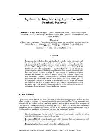
Figure 1. This figure illustrates the conceptual idea behind Function Modeling. For each raster transformation(yellow triangles) within a conventional model (CM), an intermediate raster dataset is created (green square).Intermediate raster datasets are then read into a raster object (blue ovals) and transformed to produce anotherintermediate raster dataset. Function Modeling (FM) does not create intermediate raster datasets and only stores thetype of transformation occurring to source raster datasets. When raster data are read, this technique performs thetransformations to the source datasets without creating intermediate raster datasets.Moreover, while ESRI’s libraries provide a vast set of procedures to manipulate data, comparedto the programming environment used by many statisticians and mathematical modelers, these proceduresare relatively limited to some of the more basic statistical and machine learning algorithms. In addition,the algorithms that are available in standard libraries are not directly accessible within ESRI classesbecause they are wrapped into a class requiring an input that produces a predefined output. While thiskind of encapsulation does simplify coding, it limits the use of the algorithms to the designed classworkflow. Take for example the principal component analysis (PCA) class within Spatial Analystnamespace (ESRIa, 2010, ESRIb 2010). The interface to this class requires three simple inputs (rasterbands, path to estimated parameters, and optional number of components to calculate) and produces twooutputs (a new raster surface and the estimated parameters). Within the class, the PCA algorithmcombines a number of statistical steps to generate the PCA estimates (e.g., calculating variance covariance and performing the matrix algebra to estimate Eigen values and vectors). These estimates arethen used to transform the original bands into an orthogonal raster dataset. Though simple to code andimplement for raster data, the algorithms used to estimate Eigen values and vectors within the classcannot be applied to other workflows that use different types of data (e.g., vector data). These types oflimitations significantly restrict the types of analyses that can be performed within ArcDesktop andnecessitate the development and integration of additional libraries. In this study we address the limitationsof raster spatial modeling and complex statistical and machine learning algorithms within the ArcDesktopenvironment by extending ArcMap’s functionality and creating a new modeling framework calledFunction Modeling (FM).Hogland et al. 2014. ESRI User ConferencePage 3 of 14
Methods.NET LibrariesTo address these challenges we developed a series of coding libraries that leverage the conceptsof delayed reading using Function Raster Datasets (ESRIc 2010) and integrate numeric, statistical, andmachine learning algorithms with ESRI’s ArcObjects. Combined, these libraries facilitate FM whichallows users to chain modeling steps and complex algorithms into one raster dataset or field calculationwithout writing the outputs of intermediate modeling steps to disk. Our libraries were built using anobject-oriented design, .NET framework, ESRI’s ArcObjects, ALGLIB (Sergey 2009), and Accord.net(Souza 2012). This work is easily accessible to coders and analysts through our subversion site (FSSoftware Center 2012) and ESRI toolbar add-in (RMRS 2012).The methods and procedures of our class libraries parallel many of the functions found in ESRI’sSpatial Analyst extension including focal, aggregation, resampling, convolution, remap, local, arithmetic,mathematical, logical, zonal, surface, and conditional. However, our libraries support multibandmanipulations and perform these transformations without writing intermediate or final output rasterdatasets to disk. Our spatial modeling framework focuses on storing only the manipulations occurring todatasets and applying those transformations dynamically at the time data are read, greatly reducingprocessing time and data storage requirements. In addition to including common types of rastertransformations, we have developed and integrated multiband manipulation procedures such as gray levelco-occurrence matrix (GLCM), landscape metrics, entropy and angular second moment calculations forfocal and zonal procedures, image normalization, and a wide variety of statistical and machine learningtransformations directly into this modeling framework.While the statistical and machine learning transformations can be used to build surfaces andcalculate records within a field, they do not in themselves define the relationships between response andexplanatory variables like a predictive model. To define these relationships, we built a suite of classes thatperforms a wide variety of statistical testing and predictive modeling using many of the optimizationalgorithms and mathematical procedures found within the ALGLIB (Sergey 2009) and Accord.net (Souza2012) projects. Typically, these classes use samples drawn from a population of tabular records or rastercells to test hypotheses and create generalized associations (e.g., an equation or procedure) betweenvariables of interest that are expensive to collect (i.e. response variables) and variables that are less costlyand thought to be related to the response (i.e. explanatory variables; Figure 2). While the inner workingsand assumptions of the algorithms used to develop these relationships are beyond the scope of this paper,the classes developed to utilize these algorithms within a spatial context provide coders and analysts withthe ability to easily use these techniques to define relationships and answer a wide variety of questions.Combined with FM, the sampling, equation\procedure building, and predictive surface creation workflowcan be streamlined to produce outputs that not only answer questions, but also display relationshipsbetween response and explanatory variables in a spatially explicit manner at fine resolutions across largespatial extents.Hogland et al. 2014. ESRI User ConferencePage 4 of 14
AspenFigure 2. An example of a generalized association (predictive model) between tons of above ground Aspen biomass(response) and nine explanatory variables derived from remotely sensed imagery. This relationship was developedusing a random forest algorithm and the RMRS Raster Utility coding libraries. The top graphic illustrates thefunctional relationship between biomass and the explanatory variable called “PredProbVert CONTRAST Band12”,while holding all other explanatory variables values at 20% of their sampled range. The bottom graphic depicts theimportance of each variable within the predictive model by systematically removing one variable from the modeland comparing changes in root mean squared error (RMSE).SimulationsFrom a theoretical standpoint, FM should reduce processing time and storage space associatedwith spatial modeling (i.e., less in and out reading and writing from and to disk). However, to justify theuse of FM methods, it is necessary to quantify the extent to which FM actually reduces processing andstorage space. To evaluate the efficiency gains associated with FM, we designed, ran, and recordedHogland et al. 2014. ESRI User ConferencePage 5 of 14
processing time and storage space associated with six simulations, varying the size of the raster datasetsused in each simulation. From the results of those simulations we compared and contrasted FM withconventional modeling (CM) techniques using linear regression. All CM techniques were directly codedagainst ESRI’s ArcObject Spatial Analyst classes to minimize CM processing time and provide a faircomparison.Spatial modeling scenarios within each simulation ranged from one arithmetic operation to twelveoperations that included arithmetic, logical, conditional, focal, and local type analyses (Table 1). Eachmodeling scenario created a final raster output and was run against six raster datasets ranging in size from1,000,000 to 121,000,000 total cells, incrementally increasing in size by 2000 columns and 2000 rows ateach step. Cell bit depth remained constant as floating type numbers across all scenarios and simulations.Table 1. Spatial operations used to compare and contrast Function Modeling and conventional raster modeling.Superscript values indicate the number of times an operation was used within a given model. Model number(column 1) also indicates the total number of processes performed for a given model.ModelSpatial Operation Types1Arithmetic ( )2Arithmetic ( ) & Arithmetic ( )3Arithmetic ( ), Arithmetic ( ) & Logical ( )4Arithmetic ( )2, Arithmetic ( ) & Logical ( )5Arithmetic ( )2, Arithmetic ( ), Logical ( ) & Focal (Mean,7,7)6Arithmetic ( )2, Arithmetic ( )2, Logical ( ) & Focal (Mean,7,7)7Arithmetic ( )2, Arithmetic ( )2, Logical ( ), Focal (Mean,7,7), & Conditional8Arithmetic ( )3, Arithmetic ( )2, Logical ( ), Focal (Mean,7,7), & Conditional9Arithmetic ( )3, Arithmetic ( )2, Logical ( ), Focal (Mean,7,7), Conditional, & Convolution (Sum,5,5)10Arithmetic ( )3, Arithmetic ( )3, Logical ( ), Focal (Mean,7,7), Conditional, & Convolution(Sum,5,5)Arithmetic ( )3, Arithmetic ( )3, Logical ( ), Focal (Mean,7,7), Conditional, Convolution(Sum,5,5), &11Local( )Arithmetic ( )4, Arithmetic ( )3, Logical ( ), Focal (Mean,7,7), Conditional, Convolution(Sum,5,5), &12Local( )Case studyFurthermore, to illustrate the benefits of using FM to analyze data and create predictive surfaces,we evaluated the time savings associated with a recent study in the Uncompahgre National Forest (UNF;Hogland et. al., 2014). In this study we used FM, field data, and fine resolution imagery to develop a twostage classification and estimation procedure that predicts mean values of forest characteristics across 0.5million acres at a spatial resolution of 1 m2. The base data used to create these predictions consisted ofNational Agricultural Imagery Program (NAIP) color infrared (CIR) imagery (U.S. Department ofAgriculture National Agriculture Imagery Program 2012), which contained a total of ten billion pixels forthe extent of the study area. Within this project we created no less than 365 explanatory raster surfaces(many of which represented a combination of multiple raster functions), 52 predictive models, and 64predictive surfaces at the extent and spatial resolution of the NAIP imagery 1.While it would be ideal to directly compare CM with FM for the UNF case study, ESRI’slibraries do not have procedures to perform many of the analyses and raster transformations used in thestudy, so CM was not incorporated directly into the analysis. Alternatively, to evaluate the time savingsassociated with using FM we used our simulated results and estimated the number of individual CMfunctions required to create GLCM explanatory variables and model outputs. Processing time was based1While this study initially used spatial analyst procedures (PCA and ISO cluster) and statistical SAS software tobuild predictive models, our libraries have since added these techniques, which in turn have been used to generatethe final outputs for this study.Hogland et al. 2014. ESRI User ConferencePage 6 of 14
on the number of CM functions required to produce explanatory variables and predictive surfaces. Inmany instances, multiple CM functions were required to create just one explanatory variable or finaloutput. The number of functions were then multiplied by the corresponding proportion increase inprocessing time associated with CM when compared to FM. Storage spaced was calculated based on thenumber of intermediate steps used to create explanatory variables and final outputs. In all cases the spaceassociated with intermediate outputs from CM were calculated without data compression and summed toproduce a final storage space estimate.Results.Net LibrariesLeveraging ESRI’s API, we were able to substantially reduce development time and focus ourresources on designing solutions to analytical problems. Currently, our solution contains 639 files, over70,000 lines of code, 457 classes, and 74 forms that facilitate functionality ranging from data acquisitionto raster manipulation and statistical/machine learning types of analyses. Our coding solution, RMRSRaster Utilities, contains two primary projects that consist of an ESRI Desktop class library (“esriUtil”)and an ArcMap add-in (“servicesToolBar”). The project esriUtil contains most of the functionality of oursolution, while the servicesToolBar project wraps that functionality into a toolbar accessible withinArcMap. In addition, two open source numeric class library solutions are used within our esriUtil project.These solutions, Accord.net (Souza 2012) and ALGLIB (Sergey 2009), provide access to numeric,statistical, and machine learning algorithms used to facilitate the statistical and machine learningprocedures within our classes.Our esriUtil project represents the bulk of our coding endeavor and the classes within this projectare grouped based on functionality into General Procedures, Data Acquisition, Raster Utilities, Sampling,and Statistical Procedures. General Procedures include classes that facilitate FM, batch processing,opening and closing function models, managing models, and saving FM to conventional raster datasets(e.g., Imagine file format). Data Acquisition classes streamline the use of web services to interactivelydownload and store vector and raster data. Raster Utilities classes streamline raster transformations andsummarizations and builds the underlining foundation for FM. Sampling classes focus on creatingsamples of populations and extracting values from raster datasets for those samples. Statistical Proceduresclasses summarize datasets and analyze variables within those datasets to test hypotheses and buildpredictive models.The primary classes within esriUtil include a database manipulation class (geodatabaseutily),raster manipulation class (rasterUtil), feature manipulation class (featureUtil), and multiple statistical andmachine learning classes (Statistics). The geodatabaseutility class contains 2,831 lines of code thatstreamlines vector, tabular, and raster data access and provides procedures to create vector and tabulardata along with fields within vector and tabular datasets. The rasterUtil class contains 4,258 lines of codeand 124 public procedures that focus on dynamically transforming raster datasets using raster functions.Many of these procedures reference 56 newly developed raster functions that create transformations ofraster datasets. Raster transformations for these newly developed raster functions range from surface typemanipulations to generating predictive model outputs (Table 2) and can be added to any function rasterdataset to produce a FM. The featureUtil class contains 815 lines of code and simplifies selecting featuresbased on the statistical properties of the data and exporting features to a new output. Our Statisticsnamespace contain 88 different classes with over 12,000 lines of code that performs a wide variety ofanalyses ranging from categorical data analysis to creating predictive models such as principle componentanalysis (PCA), clustering, general linear modeling (GLM), Random Forest , and Soft-max neural nets(Table 3).Hogland et al. 2014. ESRI User ConferencePage 7 of 14
Table 2. Raster transformations that can be applied to function raster datasets using the raterUtil class of the esriUtilproject.Raster DescriptionAdds, subtracts, multiplies, divides, and calculate modulus for two multiband raster datasets or a multibandraster dataset and a constant*Mathematically transform a multiband raster datasetLogical Analysis*Performs , , , , logical comparisons between to multiband raster datasets or a multiband rasterdataset and a constantConditionalAnalysis*Performs a conditional analysis using multiband raster datasets and/or constantsRemap RasterRemaps the cell values of a multiband raster datasetFocal Analysis* Performs focal analyses for a multiband raster datasetFocal Sample* Samples raster cells of a multiband raster dataset within a focal window, given defined offsets from thecentral window cellConvolutionAnalysis* Performs convolution analysis on multiband raster datasetLocal Stat Analysis* Performs local type analysis on a multiband raster datasetLinear Transform* Performs a linear transformation of a multiband raster datasetGLCM* Performs grey level co-occurrence matrix transformations on multiband raster datasetsLandscape Metrics* Performs moving window landscape metrics transformations for multiband raster datasetsCreate ConstantRaster* Creates a constant value raster datasetNull Data to value* Converts no data to a new value for multiband raster datasetSet Values to NoData* Sets specified values to no data for multiband raster datasetSet Null Value* Sets the values used for no data in a raster datasetFlip Raster* Flips multiband raster datasetsShift Raster* Shifts multiband raster datasets based on a specified number of pixelsRotate Raster* Rotates multiband raster datasets based on a specified angleCombine Raster* Combines multiband raster dataset to create a single band raster dataset of unique raster band combinationsAggregate Cells* Resamples and perform a summarization of all cells used to increase the cell sizeSlope RasterCalculates slopeCalculate AspectCalculates aspectNorthing* Converts aspect to a northing raster datasetEasting* Converts aspect to a easting raster datasetClip AnalysisClips a multiband raster dataset given either the extent of a raster dataset or the boundary of a feature classConvert Pixel TypeTransforms pixel depth for multiband raster datasetsRescale Analysis* Rescales pixel values of a multiband raster dataset to the min and max values given the defined pixel depthCreate Composite* Creates a multiband raster dataset given specified bands from multiple raster datasetsExtract Bands* Creates a multiband raster dataset by extract specified bands of a multiband raster datasetTasseled Cap* Performs a Tasseled Cap transformation (Landsat 7 coefficients)NDVI* Calculates a normalized difference vegetation index (NDVI)Resample Raster* Resamples the cell size of a multiband rasterNormalize* Brings two multiband raster datasets to a common radiometric scaleMerge Raster* Merges multiband raster datasetsCreate MosaicCreates a mosaic raster datasetFunction Modeling* Combines raster function into a function modelHogland et al. 2014. ESRI User ConferencePage 8 of 14
Zonal Statistics* Performs zonal statistics on multiband raster datasetsRegion Group* Groups regions of a multiband raster datasetBuild Raster Model* Builds predictive raster surfaces given a predictive model and explanatory raster surfacesBatch Processing* Will batch process RMRS Raster Utility commands*Identifies either new procedures or functionality not available within ESRI’s Spatial Analyst extension or ImageAnalysis Window.The servicesToolBar combines the forms and procedures within esriUtil into an organized, easilydeployed toolbar. While primarily a wrapper around the functionality contained within esriUtil,servicesToolBar provides analysts with easy access to a wide array of procedures that currently do notexist within ArcMap. Moreover, many of these procedures can be tied together in a step-like fashion tobuild multi-procedure FM and batch processes. Together, these projects facilitate a wide range ofanalytics procedures that can be applied to both vector and raster type data in a streamlined, efficientfashion.Table 3. Statistical analyses and machine learning techniques accessible to coders and analysts through the RMRSRaster Utility libraries. All statistical and machine learning procedures create a RMRS Raster Utility model that canbe used to display modeling results and predict new outcomes in raster, vector, and tabular formats.AnalysisVarianceCovarianceStratified VarianceCovarianceCompare Sample ntAdjusted AccuracyAssessmentButtonDescriptionCalculates variance covariance and correlation matrices for fields within a table or bands within a rasterCalculates stratified variance covariance and correlation matrices for fields within a table or bands within arasterCompares similar fields within two tables to determine if a sample is representative of a populationCompares the accuracy and similarity of two categorical classificationsCalculates the accuracy of a classification modelAdjusts an existing accuracy assessment by weighting accuracy based on the proportions of each categorywithin a user defined extentT-TestCompares fields within a table or bands within a raster by groups or zone, respectivePCA/SVDPerforms a single vector decomposition, principal component analysis on fields within a table or bandswithin a raster datasetCluster AnalysisPerforms K-means, Gaussian, and binary clustering on fields within a table or bands within a rasterLinear RegressionPerforms multiple linear regression using fields within a table or bands within a rasterLogistic RegressionPerforms logistic regression using fields within a table or bands within a rasterGeneralized istic RegressionPerforms general linear modeling using fields within a table or bands within a raster (supported links:identity, absolute, cauchit, inverse, inverse squared, logit, log, log log, probit, sin, and threshold)Performs multivariate linear regression using fields within a table or bands within a rasterPerforms polytomous (multinomial) logistic regression using fields within a table or bands within a rasterRandom ForestPerforms random forest classification or regression tree analysis using fields within a table or bands withina rasterSoft-max NnetPerforms soft-max neural networks classification using fields within a table or bands within a rasterFormat Zonal DataFormats the outputs of multiband Zonal Statistics (Table 2) for use in statistical machine learningtechniquesView Sample SizeEstimates sample size based on a subset of the above statistical procedures using power analysisShow Model ReportShows the outputs of the above statistical and machine learning proceduresPredict New DataCreates new fields within a tabular dataset and populates the records within that field with the predictedoutcomes based on the above statistical and machine learning proceduresDelete ModelDeletes statistical and machine learning models create in the above proceduresHogland et al. 2014. ESRI User ConferencePage 9 of 14
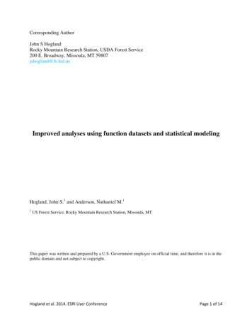
SimulationsTo evaluate the gains in efficacy of FM, we compared it with CM across six simulations. FMsignificantly reduced both processing time and storage space when compared to CM (Figures 3 and 4). Toperform all six simulations FM took 26.13 minutes and a total of 13,299.09 megabytes while CM took73.15 minutes and 85,098.27 megabytes. Theoretically, processing time and storage space associated withcreating raster data for a given model, computer configuration, set of operations, and data type should bea linear function of the total number of cells within a rater dataset and the total number of operationswithin the model:Timei (seconds) βi(cells х operations)iSpacei (megabytes) βi(cells)iwhere i denotes the technique, either FM or CM in this case. Our empirically derived FM Time and Spacemodels nicely fit the linear paradigm (R2 0.96 and 0.99, respectively). However, for the CM techniquesthe model for Time (R2 0.91) deviated slightly and the model for Space (R2 0.10) deviated significantlyfrom theoretical distributions, indicating that in addition to the modeling operations, extra operationsoccurred to facilitate raster processing and that some of those operations produced intermediate rasterdatasets, generating wider variation in time and space requirements than would be expected based onthese equations.FM and CM time equation coefficients indicate that, on average, FM reduced processing time byapproximately 278%. Model fit for FM and CM space equations varied greatly between techniques andcould not be compared reliably in the same manner. For the CM methodology, storage space appeared tovary depending on the types of operations within the model and often decreased well after the creation ofthe final dataset. This outcome is assumed to be caused by delayed removal of intermediate datasets.Overall though, FM reduced total storage space by 640% when compared to CM for the six simulations.Figure 3. Function Modeling and conventional modeling regression results for processing time.Hogland et al. 2014. ESRI User ConferencePage 10 of 14
Figure 4. Function Modeling and conventional modeling regression results for storage space.Case studyAlthough simulated results helped to quantify improvements related to using FM, the UNF casestudy illustrates these saving in a more concrete and applied manner. As described in the methods section,this project created no less than 365 explanatory raster surfaces, 52 predictive models, and 64 predictivesurfaces at the extent and spatial resolution of the NAIP imagery (202,343 ha and 1 m2, respectively). Inthis comparison, it was assumed that all potential explanatory surfaces were created for CM to facilitatesampling and statistical model building. In contrast, FM only sampled explanatory surfaces and calculatedvalues for the variables selected in the final models. For the classification stage of the UNF study, weestimated that to reproduce the explanatory variables and probabilistic outputs using CM techniques, itwould take approximately 283 processing hours on a Hewlett-Packard Eli
a GIS, 2) import that sample dataset into statistical software such as SAS (SAS 2014) or R (R 2014), 3) define a relationship (predictive model) between response and explanatory variables that can be used within a GIS to create predictive surfaces, and 4) build a representative spatial model within a GIS that