Transcription
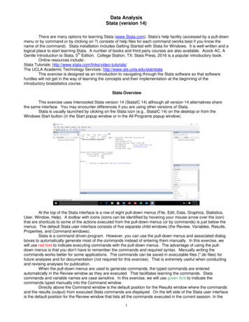
Data AnalysisStata (version 14)There are many options for learning Stata (www.Stata.com). Stata’s help facility (accessed by a pull-downmenu or by command or by clicking on ?) consists of help files for each command (works best if you know thename of the command). Stata installation includes Getting Started with Stata for Windows. It is well-written and alogical place to start learning Stata. A number of books and third party courses are also available. Acock AC. AGentle Introduction to Stata, 5th Edition. College Station, TX: Stata Press, 2016 is a popular introductory book.Online resources include:Stata Tutorials: http://www.stata.com/links/video-tutorials/The UCLA Academic Technology Services: http://www.ats.ucla.edu/stat/stataThis exercise is designed as an introduction to navigating through the Stata software so that softwarehurdles will not get in the way of learning the concepts and their implementation at the beginning of theintroductory biostatistics course.Stata OverviewThis exercise uses Intercooled Stata version 14 (StataIC 14) although all version 14 alternatives sharethe same interface. You may encounter differences if you are using other versions of Stata.Stata is usually launched by clicking on the Stata icon (e.g., StataIC 14) on the desktop or from theWindows Start button (in the Start popup window or in the All Programs popup window).At the top of the Stata interface is a row of eight pull-down menus (File, Edit, Data, Graphics, Statistics,User, Window, Help). A toolbar with icons (icons can be identified by hovering your mouse arrow over the icon)that are shortcuts to some of the actions executed from the pull-down menus (or by commands) is just below themenus. The default Stata user interface consists of five separate child windows (the Review, Variables, Results,Properties, and Command windows).Stata is a command driven program. However, you can use the pull-down menus and associated dialogboxes to automatically generate most of the commands instead of entering them manually. In this exercise, wewill use red font to indicate executing commands with the pull-down menus. The advantage of using the pulldown menus is that you don’t have to remember the commands and required syntax. Manually writing thecommands works better for some applications. The commands can be saved in executable files (*.do files) forfuture analyses and for documentation (not required for this exercise). That is extremely useful when conductingand revising analyses for publication.When the pull-down menus are used to generate commands, the typed commands are enteredautomatically in the Review window as they are executed. That facilitates learning the commands. Statacommands and variable names are case sensitive. In this exercise, we will use green font to indicate thecommands typed manually into the Command window.Directly above the Command window is the default position for the Results window where the commandsand the results (output) from executed Stata commands are displayed. On the left side of the Stata user interfaceis the default position for the Review window that lists all the commands executed in the current session. In the1
Command window, commands can be edited if an error was made or you want to repeat the command on othervariables. New variables can be inserted in the Command window by typing or by clicking on the variable namein the Variable window (on top of the Properties window to the right of the Results and Command windows).The following exercise involves reading data into Stata, then manipulating and analyzing the data. Thisexercise can be done by experienced Stata users by simply executing the tasks (commands in red and green).Less experienced users may require the supporting information provided in this tutorial.Description of the DataThe data for this exercise are from the Framingham Heart Study (www.framinghamheartstudy.org/aboutfhs/index.php ). These data are a subset of variables for men and women aged 60-62 years at study initiation.The variable names (bolded), codes, and definitions are listed below.idCase identification numberCHD01Coronary heart disease diagnosisNo evidence of CHDPre-existing CHD at study entrySBPSystolic blood pressure in mm Hg at study entryDBPDiastolic blood pressure in mm Hg at study entryCHOLSerum cholesterol in mg/100 ml at study entryCIGNumber of cigarettes smoked per day (estimated to the nearest five)death01Alive at follow upDead at follow upcausealivechdothercvdstrokecancerotherblank cellCause of deathliving at follow upcoronary heart diseaseother cardiovascular diseasestrokecancerother cause of deathmissing datagender01MaleFemaleCreating a Log FileThe Stata working directory is the default location that Stata will use for files and results unless it ischanged. Click File—Change Working Directory and indicate the folder you want for your working directory onyour computer.To have a record of your work for this exercise, you must save a log file. Log files can be stored in one oftwo formats: a text file with a .log extension or a Stata Markup and Control Language file with a .smcl extension.The *.log text files can be read and edited by any word processor program or text editor. The *.smcl files can onlybe read by the Stata program. *.smcl files can be translated to *.log files by clicking on File—Log—Translate.TO GET CREDIT FOR THIS EXERCISE, YOU MUST SUBMIT A LOGFILE. NAME YOUR LOG FILE “Stata Exercise Your Name”. YOUCAN SUBMIT EITHER AN *.smcl OR A *.log FILE.2
File—Log—Begin (you can also click the Log button in the toolbar)In the Save dialog box indicate your log’s folder at the top, the log file name (File name:), and the format (Save astype:).Click the Save button. The dialog box closes, the command you just executed is listed in the Reviewwindow and also in the Results window with some additional documentation, and log status (on) is indicated in thelower right corner of the Results window.You can make comments (descriptive information that will not be executed by the program) in log files bytyping your comment preceded by an * in the Stata Command window. You can print a log file by right clicking onthe Viewer window with the open log file and selecting Print.If you need to stop and resume this exercise, you can save the log file (it should also be automaticallysaved to your working directory when you exit the program). To add to your work later, re-enter Stata, click File—Log—Begin and insert the name of your saved log file in the dialog box. Then click on “Save” and select “Appendto existing file” in the pop up dialog box to resume adding commands and results to your log file.Keyboard Data EntryMost biomedical datasets have rows containing the data from individual subjects/cases (or other analysisunits) and columns containing different measurements or variables recorded on those cases. Data in this formatare called wide format data. Long format is used for longitudinal and clustered data and repeated measurementson the same subject. This exercise contains data in wide format.iddeathcause3
1402140314041405140600110AliveAliveCHDCHDAliveIn Stata, data are held in a spreadsheet called the Data Editor. The Data Editor is entered by clicking Data—DataEditor—Data Editor (Edit). Use your keyboard to enter the data in rows 1-5 from the table directly into the DataEditor. (Variable names will be entered later). [Tab or the right-arrow key moves you to the right, Shift-Tab or theleft-arrow key to the left, Enter or the down-arrow key down, and Shift-Enter or the up-arrow key up.] Stataautomatically assigns a variable name to each column (var1, var2, etc) when data entered. Stata distinguishestext (eg, the observations for the cause variable) from numerical data by using reddish font for the former andblack font for the latter.Variable NamesWhen you select a column in the data table, information about the variable is shown in the Variables window tothe right of the Results and Command windows. You can name or rename variables (var1, var2, etc.) here.Replace the default variable names with the appropriate names from the table above. Variable names should beshort to be efficient and descriptive enough to reduce errors when manipulating the data, conducting analyses,and reading output. Stata variable names must start with a letter, they can contain letters (variable names arecase sensitive), numbers, and the underscore but no spaces or other characters, and they can be up to 32characters in length (eight or fewer is recommended).Importing a Data FileThe data in the above table was only part of the data needed for this exercise. The complete dataconcerning id, death, and cause for all patients have been entered into an Excel file named Data-1.xls. Beforestarting to enter the new dataset, clear the Data Editor by typing clear in the Command window. Import the Excelfile, Data-1.xls. Click File—Import—Excel spreadsheet (*.xls, *.xlsx), in the Import Excel dialog box use theBrowse button to select Data-1.xls where you stored it on your computer when you downloaded the file from ourwebsite. Click on Open. Click the Import first row as variable names button, click the OK button.(Another simple way to import small Excel files is to copy/paste. Open the Excel file and select and copyall the cells. Paste what you have copied into the first/left cell in the first data row (below the first row with thevariable names) of the Stata Data Editor. If you have variable names in the first row, select Variable Names in thedialog box that asks if you want to treat the first row as variable names).Saving DataIt is prudent to regularly save your work. Closing the Data Editor does not save your data. Save these data as aStata data file (Data-1.dta):Close the Stata Data Editor (click on X in upper right corner of the Data Editor Window).File—Save AsThe Save Stata Data File dialog box pops up.At the top of the dialog box, locate the folder you want to store Data-1.dta if you don’t want your data in yourdefault folder.Make sure Stata Data (*.dta) is selected in the Save as type: box.Type Data-1 in the file name: box.Click the Save button in the lower right corner of the dialog box.You can open a previously generated and stored Stata data file (*.dta file) by clicking File—Open, or the Openbutton on the toolbar.Merging Data FilesThis exercise concerns merging two data files with different variables but the same cases in each dataset. Mergethe data in Data-1.dta with the data in Data-2.dta that you downloaded to your computer from our website. One ofthese datasets must be currently open in Stata. In this example, Data-1.dta is currently open in Stata. Thefollowing steps merge the variables in Data-1.dta with the additional variables in Data-2.dta for the casesindicated by the key variable id.4
Data—Combine datasets—Merge two datasetsThe “Merge dataset in memory with dataset on disk” dialog box opens. The key variable is the variable in bothfiles used to combine the two datasets (id).Select One-to-one on key variables as the Type of merge.Select id as the Key variables: (Match variables).Browse to select Data-2.dta as the Filename of dataset on disk. Click on Open.Click the Submit or OK button.(You can execute commands from the pull-down windows by either clicking OK or Submit in opened dialog boxes.The latter leaves the dialog box open. It is used when you want to revise your command. OK executes thecommand and closes the dialog box.)Save this merged dataset as Fram60.dta.File—Save AsThe Save Stata Data File dialog box pops up. At the top make sure you’ll save your data in the intended folderyou created for this exercise.In the Save as type: box, select Stata Data (*.dta).In the File name: box, type Fram60.dta.Click the Save button in the bottom right of the dialog box.Variable Labels and Value LabelsThe next 2 sections are optional for this computer exercise. You will need to know this for the advancedbiostatistics course and for analyzing your own data, but you won’t need this for the introductory course. You canproceed directly to the Data Exploration section (page 8) if you choose to skip this.Variable names are often insufficient to allow the datasets to be understood easily by others (or by you ifyou go back to the data after a long break). Variable labels (short definitions of the variable) and value labels(how the categories are defined) provide additional information. Variable labels are used to more fully describewhat the variables are and often include the units of measurement. They can be up to 80 characters in length;spaces or any characters can be used. Value labels are used when the numerical data entries have a textdefinition (eg, 0 and 1 for the death variable indicate Alive and Dead, respectively). Value labels are generated intwo steps. First, the numeric values and the referent words are listed and saved [eg, 0 for no and 1 for yes (thesame set could be used for more than 1 variable)] as Value Labels. Second, the Value Label list is assigned tothe variable.Click the pull down menu, Data— Variables Manager. In the Variables Manager dialog box, click theManage button next to the Value Label fill-in box. In the Manage Value Labels dialog box, click the Create Labelbutton and type a Label name for the value list you want to create (death). Then, in turn fill in each Value(number): and associated Label you want (Alive at follow-up for 0 and Dead at follow-up for 1) followed by clickingthe Add button until all the values are labeled. Click the OK button and Close the Manage Value Labels dialogbox (first step).5
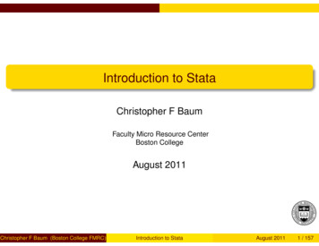
In the Variables Manager dialog box, select the death variable and type the newly created Value Label in theValue Label fill-in box and click the Apply button in order to map the named value labels to the variable (thesecond step).Close Variable Manager dialog box. Click on Apply to accept the changes you’ve made. (The Variables Manageris also used to delete variables. It can also be done directly from the spreadsheet view by selecting a columnthen right clicking and selecting Data-Drop Selected Data.)Generating New Variables and RecodingYou may need to recode variables when they are not categorized as needed for analysis. For example, CIGindicates the number of cigarettes smoked daily (rounded to the nearest 5). Recode CIG into two categories, 0for nonsmoker and 1 for smoker, and label that new variable rCIG. We will first generate the new variable rCIGand then recode that variable.Data—Create or change data—Create new variableIn the generate – Create a new variable dialog box type rCIG in the Variable name: box, int (for integer) as theVariable type:, CIG in the Specify a value or an expression box, and click Submit or OK.This creates a new variable, rCIG from the data in CIG.6
Data—Create or change data—Other variable-transformation commands—Recode categorical variableIn the recode – Recode categorical variables box select rCIG for the Variables:, type (0 0) (1/max 1) in theRequired: box, and click Submit or OK. This stipulates that a 0 in rCIG will be recoded as 0 in rCIG and anythingbetween 1 and the maximum value will be recoded as a 1. (Clicking the Examples button gives examples ofacceptable rule formats.)Recoding cause (of death) into two categories (1 for deaths from cardiovascular causes and 0 for cases still aliveand all other causes of death) involves converting the text (string) variable to a numeric variable before combiningcategories. Encoding assigns numbers to a string (text) variable. This is necessary in order to perform statisticalprocedures on string (text) variables because Stata only performs statistics on numeric variables. This commandassigns the string values as value labels to the numeric values. Stata displays them in the Data Editor as valuelabels (words) but computationally it considers them as numbers. Open the Data Editor and review the values inthe spreadsheet for CHD and death. They appear to be words but note they are blue font rather than reddish fontreserved for “true” string variable values.The cause column is displayed in a reddish font because it is a string variable that has not been encoded.Encode this variable then use the recode command to generate the two desired codes for cardiovascular death(1) and alive or non-cardiac death (0).Data—Create or change data—Other variable-transformation commands—Encode value labels from a stringvariableSelect cause as the Source string variable:Enter cvdeath (new variable that will be encoded) under New numeric variable:Click OK or Submit7
To see the numbers Stata has assigned to the cvdeath variables, use the following command after closing theData Editor (if still open).Data – Data utilities – Label utilities -- List value labelsEnter cvdeath under Labels to list:Click on Submit or OK. Stata displays the list of values for the cvdeath variable.Data—Create or change data—Other variable-transformation commands—Recode categorical variablesIn the recode – Recode categorical variables box select cvdeath for the Variables:, type (1/2 0) (3 1) (4 0)(5/6 1) in the Required: box, from the Options tab check Generate new variable, enter cvdeathyn, and clickSubmit or OK.This creates a new variable (cvdeathyn) with a value of 0 for cases with 1 or 2 or 4 for cvdeath and a value of 1for cases with 3 or 5 or 6 for cvdeath.New value labels (No for 0, Yes for 1) would need to be created for this recoded variable because the value labelsbefore the recode no longer apply to the recoded variable.Create a new variable that is the difference between systolic and diastolic blood pressure (BPdiff SBP-DBP).Data—Create or change data—Create new variableIn the generate – Create a new variable dialog box type BPdiff in the Variable name box and SBP-DBP in theSpecify a value or an expression box, float (for floating decimal point) as the Variable type:, and click Submit orOK.When you recode your data or generate new variables you should verify that your modifications are as intended.One way to verify your variables is to list your new variables and any original variables used to calculate the newvariables.Data—Describe data—List dataIn the Main tab of the list – List values of variables dialog box, select id SBP DBP BPdiff in the Variables: box andclick Submit or OK.Data ExplorationYou should explore your data before analyzing to verify the accuracy of the data and to determine how the dataare distributed. Erroneous or problematic data values need to be identified and corrected. The data in memorycommand characterizes the formatting of the data as well as other information about the variables (labels andvalue labels). The codebook command examines the data distributions. Review the following output to makesure that your data seems complete and the variables are correctly specified.Data—Describe data—Describe data in memory or in a fileSelect “In Memory” and click OKData—Describe data—Describe data contents (codebook)Leave Variables: empty and click OKNote that you may need to click on the –-more–- at the bottom left of the Results screen (or hit the Space bar) tosee all of the output. You can type set more off Enter in the Command window to disable the more function(may already be set as the default with your installation).a. Categorical variablesSome of the variables are categorical indicating the group/category to which a case belongs. Determine thefrequencies of values for the categorical variables death, cause, CHD, and CIG. You have already generated thatinformation by the codebook command above. (Scroll up in the Results pane to view what was generated foreach of these categorical variables.) Now, you will generate frequency counts for the values for each variable.Statistics—Summaries, tables, tests—Frequency Tables—Multiple one-way tablesSelect the categorical variables (click on death, cause, CHD, and CIG) you want under Categorical variables inthe dialog box. Click on Submit or OK.8
Review some of the options you can check in the Frequency Tables dialog boxes to customize the results youobtain. Review the output in the Results window. Use the window controls on the right of the Review window toexamine earlier output. The Results window only stores the most recent output. You can open your log file in theViewer window to view all your output since beginning the log file.Window—Viewer—New ViewerFile—Open, then Browse to find your log file.b. Continuous variablesSome of the variables are continuous (they measure something like blood pressure). Explore the distribution ofvalues for the variable CHOL by generating a histogram.Graphics—HistogramIn the Main tab of the histogram – Histograms for continuous and categorical variables dialog box, in the Datasection, select CHOL as the variable and Data are continuous, then select Percent in the Y-axis section. Includea line on your histogram indicating the expected normal distribution for a distribution of the same mean and SD asthe recorded CHOL variable. In the Density plots tab of the histogram – Histograms for continuous andcategorical variables dialog box select Add normal density plot. Click the Submit or OK button.Descriptive statistics are summary measures of data that describe the data. For CHOL, calculate the mean, themedian, the standard deviation, the 25th percentile (1st quartile), the 75th (3rd quartile), and the smallest (minimum)and largest (maximum) values.9
Statistics—Summaries, tables, tests—Summary and descriptive statistics—Summary statisticsIn the dialog box, select CHOL, Display additional statistics, and click the Submit or OK button.SortingWith large data sets, it can be difficult to find entries that have been identified as erroneous of missing in the datasummary. In the Data Editor (click on Data—Data Editor—Data Editor (Edit)) finding extreme values can befacilitated by sorting all the values of the variable in question. Use the Data—Sort drop down menu to sort thevariable name in question (eg, CIG). Note that Stata (like other database programs such as Access, but notnecessarily like spreadsheet programs such as Excel), sorts the entire row of data not just the selected column.Close the Data Editor.Inferential StatisticsThe primary reason for using a statistical package is to compute inferential statistics (eg, chi-squared test or ttest). In this exercise, you will perform these two common statistical tests to test the following two hypotheses:Hypothesis 1: 60-62-year-olds with CHD are more likely to die before they are 78-80 (end of follow-up) than 6062-year-olds without CHD.Data to test that hypothesis can be presented in a 2 X 2 table (cases with CHD as one row and cases withoutCHD as the other row; dead in one column and alive in the other column). Generate the 2 X 2 table with CHD asthe rows and death as the columns and calculate a chi-squared test statistic (more precisely, the Pearson’s chisquared test statistic) to test Hypothesis 1. For cases with and without CHD, indicate the percentages dead andalive.Statistics—Summaries, tables, and tests—Frequency tables—Two-way table with measures of associationIn the Main tab of the tabulate2 – Two-way tables dialog box select CHD for the Row variable: and death as theColumn variable:, check Pearson’s chi-squared under Test statistics and Within-row relative frequencies underCell contents, and click Submit or OK.10
The results are listed in the Stata Results window and the log file. The chi-square is 16.1504 with 1 degree offreedom. The significance level is listed as 0.000. The Null hypothesis is rejected; 60-62-year-olds with CHD aremore likely to die than 60-62-year-olds without CHD. To display the p value with greater precision, type return listin the Command window. It is displayed next to r(p) .Hypothesis 2: 60-62 year-olds with CHD have higher serum cholesterol levels than 60-62 year-olds without CHD.A statistical test of this hypothesis is a t-test. The t-test assumes your data are normally distributed and thevariances (dispersion of the data) are equal in the two groups. It is important to look at your data beforeconducting a statistical test. Before calculating a t-test, plot the distributions of CHOL values for the two groups ofcases, those with CHD and those without CHD.Graphics—HistogramIn the Main tab of the histogram – Histograms for continuous and categorical variables dialog box, in the Datasection, select CHOL as the variable and Data are continuous, then select Percent in the Y-axis section (shouldbe saved from when you did this before). In the By tab of the dialog box, check Draw subgraphs for uniquevalues of variables, select CHD for Variables, and click Submit or OK. You should get a histogram of thedistribution of CHOL with separate graphs for CHD yes and CHD no.Statistics—Summaries, tables, and tests—Classical tests of hypotheses—t test (mean-comparison tests)In the Main tab of the t test—(mean comparison tests) dialog box, select Two-sample using groups (because theCHOL data are all in one column), then select CHOL as the Variable name: and CHD as the Group variablename:, click Submit or OK.11
The t-test (t -1.3239) with 115 degrees of freedom and two-tailed significance level 0.1882 is consistent withaccepting the Null hypothesis.Subgroup AnalysesTest Hypothesis 2 separately for women and men.Graphics—HistogramIn the Main tab of the histogram – Histograms for continuous and categorical variables dialog box, in the Datasection, select CHOL as the variable and Data are continuous, then select Percent in the Y-axis section (shouldbe saved from when you did this before). In the By tab of the histogram – Histograms for continuous andcategorical variables dialog box, check Draw subgraphs for unique values of variables, and this time selectgender CHD for Variables, and click Submit or OK.Statistics—Summaries, tables, and tests—Classical tests of hypotheses—t test (mean-comparison tests)In the Main tab of the t-tests (mean comparison tests) dialog box, select Two-sample using groups, then selectCHOL as the Variable name: and CHD as the Group variable name:. In the by/if/in tab of the t-tests—(meancomparison tests) test dialog box, check Repeat command by groups, and select gender for the Variables thatdefine groups:, and click Submit or OK.For gender male, the t-test (t -0.7962) with 60 degrees of freedom and two-tailed significance level 0.4291 isconsistent with accepting the Null hypothesis. In contrast, for gender female, the t-test (t -2.0226) with 53degrees of freedom and two-tailed significance level 0.0482 is consistent with rejecting the Null hypothesis atthe 0.05 level of significance.Congratulations! You’re finished with the tasks in the exercise.When you exit Stata, your log file will be automatically closed and saved (you can also close it manually, File—Log—Close). The data file (changes you made) will not be saved automatically; you must select Save in thedialog box when you exit the program. You can edit a *.log file using Microsoft Notepad, Word, or otherprograms. You can delete unintended commands and results and add comments (put an * before the comment)to make your file more readable. If you created your log file as an *.scml file, you will need to translate it (File –Log – Translate) to a *.log file before you can edit it.Email your log file (*.log or *.scml) toDeborah.Garcia@uth.tmc.edu to receive credit for this exercise.12
two formats: a text file with a .log extension or a Stata Markup and Control Language file with a .smcl extension. The *.log text files can be read and edited by any word processor program or text editor. The *.smcl files can only be read by the Stata program. *.smcl files can be translated to *.log files by clicking on File—Log—Translate.