Transcription
1 Hierarchical Indexing forOut-of-Core Access to Multi-Resolution DataValerio Pascucci and Randall J. FrankCenter for Applied Scientific Computing, Lawrence Livermore National Laboratory.Summary. Increases in the number and size of volumetric meshes have popularized the useof hierarchical multi-resolution representations for visualization. A key component of theseschemes has become the adaptive traversal of hierarchical data-structures to build, in realtime, approximate representations of the input geometry for rendering. For very large datasetsthis process must be performed out-of-core. This paper introduces a new global indexingscheme that accelerates adaptive traversal of geometric data represented with binary trees byimproving the locality of hierarchical/spatial data access. Such improvements play a criticalrole in the enabling of effective out-of-core processing.Three features make the scheme particularly attractive: (i) the data layout is independentof the external memory device blocking factor, (ii) the computation of the index for rectilineargrids is implemented with simple bit address manipulations and (iii) the data is not replicated,avoiding performance penalties for dynamically modified data.The effectiveness of the approach was tested with the fundamental visualization technique of rendering arbitrary planar slices. Performance comparisons with alternative indexingapproaches confirm the advantages predicted by the analysis of the scheme.1.1 IntroductionThe real time processing of very large volumetric meshes introduces unique algorithmic challenges due to the impossibility of fitting the data in the main memory of a computer. The basicassumption (RAM computational model) of uniform-constant-time access to each memorylocation is not valid because part of the data is stored out-of-core or in external memory. Theperformance of many algorithms does not scale well in the transition from the in-core to theout-of-core processing conditions. This performance degradation is due to the high frequencyof I/O operations that start dominating the overall running time (trashing).Out-of-core computing [22] addresses specifically the issues of algorithm redesign anddata layout restructuring, necessary to enable data access patterns with minimal out-of-coreprocessing performance degradation. Research in this area is also valuable in parallel anddistributed computing, where one has to deal with the similar issue of balancing processingtime with data migration time.The solution of the out-of-core processing problem is typically divided into two parts:(i) algorithm analysis to understand its data access patterns and, when possible, redesignto maximize their locality;(ii) storage of the data in secondary memory with a layout consistent with the accesspatterns of the algorithm, amortizing the cost individual I/O operations over several memoryaccess operations.In the case of hierarchical visualization algorithms for volumetric data, the 3D input hierarchy is traversed to build derived geometric models with adaptive levels of detail. The
2Valerio Pascucci and Randall J. Frankshape of the output models are then modified dynamically with incremental updates of theirlevel of detail. The parameters that govern this continuous modification of the output geometry are dependent on runtime user interaction, making it impossible to determine, a priori,what levels of detail will be constructed. For example, parameters can be external, such asthe viewpoint of the current display window or internal, such as the isovalue of an isocontouror the position of an orthogonal slice. The general structure of the access pattern can be summarized into two main points: (i) the input hierarchy is traversed coarse to fine, level by levelso that the data in the same level of resolution is accessed at the same time and (ii) withineach level of resolution the data is mainly traversed coherently in regions that are in closegeometric proximity.In this paper we introduce a new static indexing scheme that induces a data layout satisfying both requirements (i) and (ii) for the hierarchical traversal of -dimensional regular grids.The scheme has three key features that make it particularly attractive. First, the order of thedata is independent of the out-of-core blocking factor so that its use in different settings (e.g.local disk access or transmission through a network) does not require any large data reorganization. Second, conversion from the standard Z-order indexing to the new indexing schemecan be implemented with a simple sequence of bit-string manipulations making it appealingfor a possible hardware implementation. Third, there is no data replication, avoiding any performance penalty for dynamic updates or any inflated storage typical of most hierarchical andout-of-core schemes.Beyond the theoretical interest in developing hierarchical indexing schemes for -dimensional space filling curves, our approach targets practical applications in out-of-core visualization algorithms. In this paper, we report algorithmic analysis and experimental results forthe case of slicing large volumetric datasets.The remainder of this paper is organized as follows. Section 1.2 discusses briefly previous work in related areas. Section 1.3 introduces the general framework for the computationof the new indexing scheme. Section 1.4 discusses the implementation of the approach forbinary tree hierarchies. Section 1.5 analyzes the application of the scheme for progressivecomputation of orthogonal slices reporting experimental timings for memory mapped files.Section 1.6 presents the structure of the I/O system and practical results obtained with compressed data. Concluding remarks and future directions are discussed in section 1.7.1.2 Related Previous WorkExternal memory algorithms [22], also known as out-of-core algorithms, have been rising tothe attention of the computer science community in recent years as they address, systematically, the problem of the non-uniform memory structure of modern computers (e.g. L1/L2cache, main memory, hard disk, etc). This issue is particularly important when dealing withlarge data-structures that do not fit in the main memory of a single computer since the access time to each memory unit is dependent on its location. New algorithmic techniquesand analysis tools have been developed to address this problem in the case of geometric algorithms [1,2,9,15] and scientific visualization [4,8]. Closely related issues emerge in thearea of parallel and distributed computing where remote data transfer can become a primarybottleneck in the computation. In this context space filling curves are often used as a toolto determine, very quickly, data distribution layouts that guarantee good geometric locality [10,18,20]. Space filling curves [21] have been also used in the past in a wide varietyof applications [3] because of their hierarchical fractal structure as well as for their well
1Hierarchical Indexing for Out-of-Core Access to Multi-Resolution Data(a)(b)(c)(d)(e)(f)(g)(h)(i)(j)3Fig. 1.1. (a-e) The first five levels of resolution of the 2D Lebesgue’s space fillingcurve. (f-j) The first five levels of resolution of the 3D Lebesgue’s space fillingcurve.known spatial locality properties. The most popular is the Hilbert curve [11] which guarantees the best geometric locality properties [19]. The pseudo-Hilbert scanning order [7,6,12]generalizes the scheme to rectilinear grids that have different number of samples along eachcoordinate axis.Recently Lawder [13,14] explored the use of different kinds of space filling curves todevelop indexing schemes for data storage layout and fast retrieval in multi-dimensionaldatabases.Balmelli at al. [5] use the Z-order (Lebesque) space filling curve to navigate efficiently aquad-tree data-structure without using pointers.In the approach proposed here a new data layout is used to allow efficient progressiveaccess to volumetric information stored in external memory. This is achieved by combininginterleaved storage of the levels in the data hierarchy while maintaining geometric proximitywithin each level of resolution (multidimensional breadth first traversal). One main advantage is that the resulting data layout is independent of the particular adaptive traversal of thedata. Moreover the same data layout can be used with different blocking factors making itbeneficial throughout the entire memory hierarchy.1.3 Hierarchical Subsampling FrameworkThis section discusses the general framework for the efficient definition of a hierarchy overthe samples of a dataset.Consider a set of elements decomposed into a hierarchy of levels of resolution such that:
4Valerio Pascucci and Randall J. Frankwhere is said to be coarser than if a cardinality functionholds: . The order of the elements in is defined by . This means that the following identity always where square brackets are used to index an element in a set.One can define a derived sequence ¼ of sets ¼ as follow: ¼ ¼ ¼ ¼ ¼ is a partitioning of can be defined on the basis of the where formally . The sequenceA derived cardinality function ¼ following two properties: ¼ ¼ ¼ ¼ ¼ ¼ ¼ If the original function has strong locality properties when restricted to any level of resolution then the cardinality function ¼ generates the desired global index for hierarchicaland out-of-core traversal. The scheme has strong locality if elements with with close indexare also close in geometric position. This locality properties are well studied in [17].The construction of the function can be achieved in the following way: (i) determine thenumber of elements in each derived set ¼ and (ii) determine a cardinality function ¼¼¼ restriction of ¼ to each set ¼ . In particular if is the number of elements of ¼ one can predetermine the starting index of the elements in a given level of resolution by buildingthe sequence of constants with (1.1)Next, one must determine a set of local cardinality functions ¼¼that: ¼ ¼ ¼ so¼¼ (1.2) The computation of the constants can be performed in a preprocessing stage so that thecomputation of ¼ is reduced to the following two steps:given determine its level of resolution (that is the such thatcompute ¼¼and add it to ¼ These two steps must be performed very efficiently as they will be executed repeatedly at runtime. The following section reports a practical realization of this scheme for rectilinear cubegrids in any dimension.
1Hierarchical Indexing for Out-of-Core Access to Multi-Resolution Data(a)(b)5(c)(d)(e)(f)(g)(h)(i)Fig. 1.2. The nine levels of resolution of the binary tree hierarchy defined by therectilinear grid. The coarsest level of2D space filling curve applied onresolution (a) is a single point. The number of points that belong to the curve at anylevel of resolution (b-i) is double the number of points of the previous level. 1.4 Binary Trees And the Lebesgue Space Filling CurveThis section reports the details on how to derive from the Z-order space filling curve the localcardinality functions ¼¼ for a binary tree hierarchy in any dimension and its remapping to thenew index ¼ .1.4.1 Indexing the Lebesgue Space Filling CurveThe Lebesgue space filling curve, also called Z-order space filling curve for its shape in the 2Dcase, is depicted in figure 1.1(a-e). The Z-order space filling curve can be defined inductivelyby a base Z shape of size (figure 1.1a) whose vertices are replaced each by a Z shape of size (figure 1.1b). The vertices obtained are then replaced by Z shapes of size (figure 1.1c)and so on. In general, the level of resolution is defined as the curve obtained by replacing level of resolution with Z shapes of size . The 3D version of thisthe vertices of the space filling curve has the same hierarchical structure with the only difference that the basicZ shape is replaced by a connected pair of Z shapes lying on the opposite faces of a cube asshown in Figure 1.1(f). Figure 1.1(f-j) show five successive refinements of the 3D Lebesgue
6Valerio Pascucci and Randall J. Frankspace filling curve. The -dimensional version of the space filling curve has also the samehierarchical structure, where the basic shape (the Z of the 2D case) is defined as a connected-dimensional basic shapes lying on the opposite faces of a -dimensional cube.pair of The property that makes the Lebesgue’s space filling curve particularly attractive is theeasy conversion from the indices of a -dimensional matrix to the 1D index along thecurve. If one element has -dimensional reference its 1D reference is built byinterleaving the bits of the binary representations of the indices . In particular if is represented by the string of bits (with ) then the 1D referenceof is represented the string of bits . 00000011248121242 levelZ-order index (2 levels)Z-order index (3 levels)Z-order index (4 levels)Z-order index (5 levels)hierarchical index 3 43613 5 712 2 6 10 14 1 3 5 7 9 11 13 153 4 5 6 7 8 9 10 11 12 13 14 15Table 1.1. Structure of the hierarchical indexing scheme for binary tree combinedwith the order defined by the Lebesgue space filling curve.The 1D order can be structured in a binary tree by considering elements of level , thosethat have the last bits all equal to 0. This yields a hierarchy where each level of resolutionhas twice as many points as the previous level. From a geometric point of view this meansthat the density of the points in the -dimensional grid is doubled alternatively along eachcoordinate axis. Figure 1.2 shows the binary hierarchy in the 2D case where the resolution ofthe space filing curve is doubled alternatively along the and axis. The coarsest level (a) isa single point, the second level (b) has two points , the third level (c) has four points (formingthe Z shape) and so on.1.4.2 Index RemappingThe cardinality function discussed in section 1.3 for a binary tree case has the structure shownin table 1.1. Note that this is a general structure suitable for out-of-core storage of static binarytrees. It is independent of the dimension of the grid of points or of the Z-order space fillingcurve.The structure of the binary tree defined on the Z-order space filling curve allows one toeasily determine the three elements necessary for the computation of the cardinality. Theyare: (i) the level of an element, (ii) the constants of equation (1.1) and (iii) the localindices ¼¼ . - if the binary tree hierarchy has levels then the element of Z-order index in the order belongs to the level , where is the number of trailing zeros in the binaryrepresentation of ;
1Hierarchical Indexing for Out-of-Core Access to Multi-Resolution Data7Step 1: shift right with incoming bit set to 1Incoming bitShiftOutgoing bit00101101001001011010 01Loop: While the outgoing bit is zeroshift right with incoming bit set to 0Shift0100101101 00010010110 100100101100(a)(b)Fig. 1.3. (a) Diagram of the algorithm for index remapping from Z-order to the hierarchical out-of-core binary tree order. (b) Example of the sequence of shift operations necessary to remap an index. The top element is the original index the bottomis the output remapped index. - the total number of elements in the levels coarser than , with ;¼¼ - if an element has index , is with and belongs to the set ¼ then must be an odd number,by definition of . Its local index is then:¼¼ ·½ The computation of the local index ¼¼ can be explained easily by looking at the bottomright part of table 1.1 where the sequence on indices (1 , 3 , 5 , 7 , 9 , 11 ,13 ,15) needs tobe remapped to the local index (0 ,1 ,2 ,3 ,4 ,5 ,6 ,7 ). The original sequence is made of aconsecutive series of odd numbers. A right shift of one bit (or rounded division by two) turnsthem into the desired sequence.These three elements can be put together to build an efficient algorithm that computes the¼¼ in the two steps shown in the diagram of Figure 1.3:hierarchical index ¼ ;1. set to 1 the bit in position 2. shift to the right until a 1 comes out of the bit-string.Clearly this diagram could have a very simple and efficient hardware implementation. Thesoftware C version can be implemented as follows:inline adhocidex remap(register adhocindex i){i last bit mask; // set leftmost onei / i&-i;// remove trailing zerosreturn (i 1);// remove rightmost one}This code would work only on machines with two’s complement representation of numbers.In a more portable version one needs to replace i / i&-i with i / i&(( i) 1).Figure 1.4 shows the data layout obtained for a 2D matrix when its elements of arereordered following the index ¼ . The data is stored in this order and divided into blocks ofconstant size. The inverse image of such decomposition has the first block corresponding tothe coarsest level of resolution of the data. The following blocks correspond to finer and finerresolution data that is distributed more and more locally.
8Valerio Pascucci and Randall J. FrankB0 B1B2 B3B4 B5 B6 B7 B8 B9 B10 B11B0B4B8B1B5B9B2B6B10B3B7B11Fig. 1.4. Data layout obtained for a 2D matrix reorganized using the index ¼ (1Darray at the top). The inverse image of the block decomposition of the 1D arrayis shown below. Each gray region shows where the block of data is distributed inthe 2D array. In particular the first block is the set of coarsest levels of the datadistributed uniformly on the 2D array.The next block is the next level of resolutionstill covering the entire matrix. The next two levels are finer data covering each halfof the array. The subsequent blocks represent finer resolution data distributed withincreasing locality in the 2D array.1.5 Computation of Planar SlicesThis section presents some experimental results based on the simple, fundamental visualization technique of computing orthogonal slices of a 3D rectilinear grid. The slices can becomputed at different levels of resolution to allow real time user interactivity independent ofthe size of the dataset. The data layout proposed here is compared with the two most commonarray layouts: the standard row major structure and the brick decomposition of thedata. Both practical performance tests and complexity analysis lead to the conclusion that thedata layout proposed allows one to achieve substantial speedup both when used at coarse resolution and traversed in a progressive fashion. Moreover no significant performance penaltyis observed if used directly at the highest level of resolution. 1.5.1 External Memory Analysis for Axis-Orthogonal SlicesThe out-of-core analysis reports the number of data blocks transferred from disk under theassumption that each block of data of size is transferred in one operation independently ofhow much data in the block is actually used. At fine resolution the simple row major arraystorage achieves the best and worst performances depending on the slicing direction. If theoverall grid size is and the size of the output is , then the best slicing direction requires oneto load data blocks (which is optimal) but the worst possible direction requires oneto load blocks (for ¿ ). In the case of simple data blocking (which¿ ) the number of blocks of data loaded at fine resolutionhas best performance for are Ô¿ ¾ . Note that this is much better than the previous case because the performanceis close to (even if not) optimal, and independent of the particular slicing direction. For a ¾ for ¿ . This means thatsubsampling rate of the performance degrades to Ô¿ ¾at coarse subsampling, the performance goes down to . The advantage of the schemeproposed here is that independent of the level of subsampling, each block of data is used for a
1Hierarchical Indexing for Out-of-Core Access to Multi-Resolution Data1e 099binary tree with Z-order remapping32*32*32 blocks1e 081e 07data loaded1e 06100000100001000100101110100100010000Sub-sampling frequency (1 full resolution, 2 every other element, .).Fig. 1.5. Maximum data loaded from disk (vertical axis) per slice computed depending onthe level of subsampling (horizontal axis) for an 8G dataset. (a) Comparison of the brick decomposition with the binary tree with Z-order remapping scheme proposed here. The valueson the vertical axis are reported in logarithmic scale to highlight the difference in orders ofmagnitude at any level of resolution. portion of ¿ so that, independently of the slicing direction and subsampling rate, the worstcase performance is Ô¿ ¾ . This implies that the fine resolution performance of the schemeis equivalent to the standard blocking scheme while at coarse resolutions it can get orders ofmagnitude better. More importantly, this allows one to produce coarse resolution outputs atinteractive rates independent of the total size of the dataset.A more accurate analysis can be performed to take into account the constant factors thatare hidden in the big notation and determine exactly which approach requires one to loadinto memory more data from disk. We can focus our attention to the case of a 8GB datasetwith disk pages on the order of 32KB each as shown in diagram of Figure 1.5. One slice ofblocksdata is 4MB in size. In the brick decomposition case, one would useof 32KB. The data loaded from disk for a slice is 32 times larger than the output, that is128MB bytes. As the subsampling increases up to a value of 32 (one sample out of 32) thebrick needs to be loadedamount of data loaded does not decrease because eachcompletely. At lower subsampling rates, the data overhead remains the same: the data loadedis 32768 times larger than the data needed. In the binary tree with Z-order remapping thedata layout is equivalent to a -tee constructing the same subdivision of an octree. Thismaps on the slice to a -tree with the same decomposition as a quadtree. The data loadedis grouped in blocks along the hierarchy that gives an overhead factor in number of blocks of while each block is 16KB. This means that the total amount of data loaded at fine resolution is the same. If the block size must be equal to 32KB the datalocated would twice as much as the previous scheme. The advantage is that each time thesubsampling rate is doubled the amount of data loaded from external memory is reduced bya factor of four. 1.5.2 Tests with Memory Mapped FilesA series of basic tests were performed to verify the performance of the approach using ageneral purpose paging system. The out-of-core component of the scheme was implemented
10Valerio Pascucci and Randall J. Frank Grid500Mhz Intel PIII, 128MB RAMbinary tree with Z-order remapping16x16x16 bricksarray order - (j,k) plane slicesarray order - (j,i) plane slices10.10.010.0010.00011e-0510slice computation time in secondsaverage slice computation time in seconds10 Grid300Mhz MIPS R12000, 600MB RAMbinary tree with Z-order remapping16x16x16 bricksarray order - (j,k) plane slicearray order - (j,i) plane slice10.10.010.0010.00011e-05110100subsampling rate (1 full resolution, 2 every other element, .).1101001000subsampling rate (1 full resolution, 2 every other element, .).(a)(b)Fig. 1.6. Two comparisons of slice computation times of four different data layout schemes.The horizontal axis is the level of subsampling of the slicing scheme (test at the finest resolution are on the left).simply by mapping a 1D array of data to a file on disk using the mmap function. In this waythe I/O layer is implemented by the operating system virtual memory subsystem, paging inand out a portion of the data array as needed. No multi-threaded component is used to avoidblocking the application while retrieving the data. The blocks of data defined by the systemare typically 4KB. Figure 1.6(a) shows performance tests executed on a Pentium III Laptop.The proposed scheme shows the best scalability in performance. The brick decompositionscheme with chunks of regular grids shows the next best compromise in performance.The row major storage scheme has the worst performance compromise because ofits dependency on the slicing direction: best for plane slices and worst for planeslices. Figure 1.6(b) shows the performance results for a test on a larger, 8GB dataset, run onan SGI Octane. The results are similar. 1.6 Budgeted I/O and Compressed StorageA portable implementation of the indexing scheme based on standard operating system I/Oprimitives was developed for Unix and Windows. This implementation avoids several application level usability issues associated with the use of mmap. The implemented memoryhierarchy consists of a fixed size block cache in memory and a compressed disk format withassociated meta-data. This allows for a fixed size runtime memory footprint, required byapplications.The input to this system is a set of sample points, arbitrarily located in space (in ourtests, these were laid out as a planar grid) and their associated level in the index hierarchy.Points are converted into a virtual block number and a local index using the hierarchical Zorder space filling curve. The block number is queried in the cache. If the block is in thecache, the sample for the point is returned, otherwise, an asynchronous I/O operation for thatblock is added to an I/O queue and the point marked as pending. Point processing continuesuntil all points have been resolved (including pending points) or the system exceeds a userdefined processing time limit. The cache is filled asynchronously by I/O threads which read
1Hierarchical Indexing for Out-of-Core Access to Multi-Resolution ge Slice Computation Time (s)1010.10.010.0011248Subsampling Rate163264 Fig. 1.7. Average slice computation time forsample slices on a Linux laptop with a IntelPentium III at 500Mhz using a 20MB fixed data cache. Results are given for two differentplane access patterns R1 and T2 as well as three different data layouts BIT, BLK and ARR.The input data grid was compressed blocks from disk, decompress them into the cache, and resolve any sample pointspending on that cache operation.The implementation was testing using the same set of indexing schemes noted in theprevious section: (BIT) our hierarchical space filling curve, (BLK) decomposition of the datain cubes of size equal to the disk pages and (ARR) storage of the data as a standard row major) time-step of the PPM dataset [16]array. The dataset was one 8GB (shown in Figure 1.11 (same results were achieved with the visible female dataset shown inFigure 1.12). Since the dataset was not a power of two so it was conceptually embedded in grid and reordered. The resulting 1D array was blocked into 64KB segments andacompressed using zlib. Entirely empty blocks resulting from the conceptual embedding werenot stored as they would never be accessed. The re-ordered, compressed data was around 6percent of the original dataset size, including the extra padding.Two different slicing patterns were considered. Test R1 is a set of one degree rotationsover each primary axis. Test T1 is a set of translations of the slice plane parallel to eachprimary axis, stepping throught every slice sequentially. Slices were sampled at various levelsof sampling resolution.In the baseline test on a basic PC platform, shown in Figure 1.7, with a very limited cacheallocation, the proposed indexing scheme was clearly superior (by orders of magnitude), particularly as the sampling factor was increased. Our scheme allows one to maintain real-timeinteraction rates for large datasets using very modest resources (20MB).We repeated the same test on an SGI Onyx2 system with higher performance disk arrays, the results are shown in Figure 1.8. The results are essentially equivalent, with slightlybetter performance being achived at extreme sampling levels on the SGI. Thus, the even thehardware requirements for the algorithm are very conservative.To test the scalability of the algorithm, we ran tests with increased output slice size andinput volume sizes. When the number of slice samples was increased by a factor of four(Figure 1.9) we note that our BIT scheme is the only one that scales running times linearlywith the size of the output for subsampling rates of two or higher.
12Valerio Pascucci and Randall J. e Slice Computation Time (s)1010.10.010.0010.00011248Subsampling Rate163264 Fig. 1.8. Average slice computation time forsample slices on an SGI Onyx2 with300Mhz MIPS R12000 CPUs using a 20MB fixed data cache. Results are given for twodifferent plane access patterns R1 and T2 as well as three different data layouts BIT, BLK.and ARR. The input data grid was 1000R1-BITR1-BLKR1-ARRT1-BITT1-BLKT1-ARRAverage Slice Computation Time (s)1001010.10.010.0010.00011248163264Subsampling Rate Fig. 1.9. Average slice computation time forsample slices on an SGI Onyx2 with300Mhz MIPS R12000 CPUs using a 20MB fixed data cache. Results are given for twodifferent plane access patterns R1 and T2 as well as three different data layouts BIT, BLK.and ARR. The input data grid was grid) formed by replicating the 8GBFinally, a 0.5TB dataset (timestep 64 times was run on the same SGI Onyx2 system using a larger 60MB memorycache. Results are shown in Figure 1.10. Interactive rat
of hierarchical multi-resolution representations for visualization. A key component of these schemes has become the adaptive traversal of hierarchical data-structures to build, in real time, approximate representations of the input geometry for rendering. For very large datasets this process must be performed out-of-core.