WIXLIB

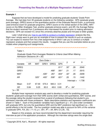
Presenting the Results of a Multiple Regression Analysis Example 1Suppose that we have developed a model for predicting graduate students’ Grade PointAverage. We had data from 30 graduate students on the following variables: GPA (graduate gradepoint average), GREQ (score on the quantitative section of the Graduate Record Exam, a commonlyused entrance exam for graduate programs), GREV (score on the verbal section of the GRE), MAT(score on the Miller Analogies Test, another graduate entrance exam), and AR, the Average Ratingthat the student received from 3 professors who interviewed the student prior to making admissiondecisions. GPA can exceed 4.0, since this university attaches pluses and minuses to letter grades.Later I shall show you how to use SAS to conduct a multiple regression analysis like this.Right now I simply want to give you an example of how to present the results of such an analysis.You can expect to receive from me a few assignments in which I ask you to conduct a multipleregression analysis and then present the results. I suggest that you use the examples below as yourmodels when preparing such assignments.Table 1.Graduate Grade Point Averages Related to Criteria Used When MakingAdmission Decisions (N 30).Zero-Order rVariableARMAT QGREQGREVMATAR.525*GPAIntercept -1.738MeanSD*p .053.5767.00575.3565.3 3.310.849.2583.048.6 0.60R2 .64*Multiple linear regression analysis was used to develop a model for predicting graduatestudents’ grade point average from their GRE scores (both verbal and quantitative), MAT scores, andthe average rating the student received from a panel of professors following that student’s preadmission interview with those professors. Basic descriptive statistics and regression coefficients areshown in Table 1. Each of the predictor variables had a significant (p .01) zero-order correlationwith graduate GPA, but only the quantitative GRE and the MAT predictors had significant (p .05)partial effects in the full model. The four predictor model was able to account for 64% of the variancein graduate GPA, F(4, 25) 11.13, p .001, R2 .64, 90% CI [.35, .72].Based on this analysis, we have recommended that the department reconsider requiring theinterview as part of the application procedure. Although the interview ratings were the single best Copyright 2018, Karl L. Wuensch - All rights reserved.MultReg-WriteUp.docx

predictor, those ratings had little to offer in the context of the GRE and MAT scores, and obtainingthose ratings is much more expensive than obtaining the standardized test scores. We recognize,however, that the interview may provide the department with valuable information which is notconsidered in the analysis reported here, such as information about the potential student’s researchinterests. One must also consider that the students may gain valuable information about us duringthe interview, information which may help the students better evaluate whether our program is reallythe right one for ------------In the table above, I have used asterisks to indicate which zero-order correlations and betaweights are significant and to indicate that the multiple R is significant. I assume that the informedreader will know that if a beta is significant then the semipartial r and the unstandardardized slope arealso significant. Providing the unstandardized slopes, and intercept is optional, but recommended insome cases – for example, when the predictors include dummy variables or variables for which theunit of measure is intrinsically meaningful (such as pounds or inches), then unstandardized slopesshould be reported. One should almost always provide either the beta weights or the semipartials orboth.If there were more than four predictors, a table of this format would get too crowded. Theunivariate statistics and zero order correlations between predictors could be presented in one tableand the statistics involving unique effects in another, like this:Table 2.Graduate Grade Point Averages Related to CriteriaUsed When Making Admission Decisions (N 30).Zero-Order rVariableARMATGREV 405*.508*.621*565.33.31MATARMean3.5767.00575.3SD*p .050.849.2583.048.6 0.60

Table 3.Multiple Regression Predicting Graduate Grade Point AveragesPredictorZero-orderr 4*.32*.26.0209AR.621*.20.15.1442Note. Exact p values are for the unique effects of the predictors.*p .05Notice that I have included the zero-order correlation coefficients. Having both the zero-ordercorrelation coefficients and the beta weights (or the semipartial correlation coefficients) helps thereader judge the extent of the effects of redundancy or of suppressor effects.When you have reliability estimates for several of the variables, they can be included on themain diagonal of the correlation matrix, like this (from Moyer, F. E., Aziz, S., & Wuensch, K.L. (2017). From workaholism to burnout: Psychological capital as a mediator. International Journalof Workplace Health Management, 10, 213-227. doi: 10.1108/IJWHM-10-2016-0074):

Table 1.Descriptive Statistics and .54**Range29 - 14524 - 1200 - 540 - 480 - SD17.9612.2312.507.465.4511.718.461.658.65Note. N 400. Entries on the main diagonal are Cronbach’s alphas. WAQ Workaholism Analysis Questionnaire; PCQ Psychological Capital Questionnaire; EE Emotional Exhaustion subscale; PA Personal Accomplishment subscale;DE Depersonalization subscale*p .05, **p .001.Example 2Here is another example, this time with a sequential multiple regression analysis. Additionalanalyses would follow those I presented here, but this should be enough to give you the basic idea.Notice that I made clear which associations were positive and which were negative. This is notnecessary when all of the associations are positive (when someone tells us that X and Y arecorrelated with Z we assume that the correlations are positive unless we are told otherwise).

ResultsComplete data1 were available for 389 participants. Basic descriptive statistics and values ofCronbach alpha are shown in Table 1Table 3Basic Descriptive Statistics and Cronbach AlphaMVariableSDαSubjective Well Being24.065.65.84Positive Affect36.415.67.84Negative Affect20.725.57.823.312.36.66Rosenberg Self Esteem40.626.14.86Contingent Self Esteem48.998.52.84Perceived Social Support84.528.39.91Social Network Diversity5.871.4519.397.45SJAS-Hard Driving/CompetitiveNumber of Persons in Social NetworkThree variables were transformed prior to analysis to reduce skewness. These includedRosenberg self esteem (squared), perceived social support (exponentiated), and number of personsin social network (log). Each outcome variable was significantly correlated with each other outcomevariable. Subjective well being was positively correlated with PANAS positive (r .433) andnegatively correlated with PANAS negative (r -.348). PANAS positive was negatively correlatedwith PANAS negative (r -.158). Correlations between the predictor variables are presented in Table2.Table 4Correlations Between Predictor 76.283ND.660**p .051Data available in Hoops.sav file on my SPSS Data Page. Intellectual property rights belong to Anne S. Hoops.

A sequential multiple regression analysis was employed to predict subjective well being. Onthe first step SJAS-HC was entered into the model. It was significantly correlated with subjective wellbeing, as shown in Table 3. On the second step all of the remaining predictors were enteredsimultaneously, resulting in a significant increase in R2, F(5, 382) 48.79, p .001. The full model R2was significantly greater than zero, F(6, 382) 42.49, p .001, R2 .40, 90% CI [.33, .45]. As shownin Table 3, every predictor had a significant zero-order correlation with subjective self esteem. SJASHC did not have a significant partial effect in the full model, but Rosenberg self esteem, contingentself esteem, perceived social support, and number of persons in social network did have significantpartial effects. Contingent self esteem functioned as a suppressor variable. When the otherpredictors were ignored, contingent self esteem was negatively correlated with subjective well being,but when the effects of the other predictors were controlled it was positively correlated with subjectivewell being.Pedagogical Note. In every table here, I have arranged to have the column of zero-ordercorrelation coefficients adjacent to the column of Beta weights. This makes it easier to detect thepresence of suppressor effects.Table 5Predicting Subjective Well BeingPredictorSJAS-Hard Driving Competitive r95% CI for -.035.131*.03, .23Rosenberg Self Esteem.561*.596*.53, .66Contingent Self Esteem.092*-.161*-.26, -.06Perceived Social Support.172*.426*.34, .50.134*.04, .23.221*.12, .31Network Diversity-.089Number of Persons in Network.107**p .05 Fair Use of this DocumentReturn to Wuensch’s Stats Lessons PageCopyright 2018, Karl L. Wuensch - All rights reserved.

Later I shall show you how to use SAS to conduct a multiple regression analysis like this. Right now I simply want to give you an example of how to present the results of such an analysis. You can expect to receive from me a few assignments in which I ask you to conduct a multiple regression analysis and then present the results.