Transcription
2015PS User Guide SeriesModeling Seismic DataPrepared ByChoon B. Park, Ph.D.January 2015
Modeling Seismic DataTable of ContentsPage1.Overview22.Importing Input Data43.Data Acquisition53.1 Seismic Source53.23.1.1 Type53.1.2 Wavelet63.1.3 Location7Recording83.2.1 Source/Receiver (SR) Array83.2.2 Recording 2Curve146.Output157.Multi-Value Run168.Execute Modeling and Outputs199.References211
Modeling Seismic Data1. OverviewThis module generates a multichannel seismic record from a layered-earth model (*.LYR) byincorporating an impulsive seismic source and multichannel recording configuration. The input model(*.LYR) consists of both elastic and inelastic properties of material assigned into each (laterallyhomogeneous) layer of a specific thickness (h); the elastic properties include compressional (Vp) andshear-wave (Vs) velocities and density ( ), and the inelastic properties include the attenuation (quality)factors (Qp and Qs) for the P and S waves.The modeling algorithm is based on the reflectivity method in its original codes developed by Fuchs andMuller (1971), provided by Dr. Klaus Holliger at the Swiss Federal Institute of Technology and Dr.Michael Roth at the Norwegian Seismic Array (NORSAR). Dr. Adam O'Neill at Kyoto University thenaltered and recompiled the codes to produce a DOS executable ("ss4exe.exe") that has been shared(with a readme file) among researchers in the field of seismology. Special acknowledgments go to all ofthem, especially to Dr. O'Neill.The reflectivity modeling provides the most realistic MASW seismic data for the following three reasons.First, in theory, each MASW record represents a 1-D (depth) measurement of subsurface materials andthe reflectivity modeling is truly a 1-D algorithm based on the laterally homogeneous medium. Second,surface waves are considered, from theoretical perspectives, as being generated through a complicatedinterference of reflections and refractions of (pure and mode converted) P and S waves and thereflectivity method is known to model such wave phenomena in a stratified medium in the mostaccurate manner at a relatively low computation cost. Lastly, the modeling can incorporate not onlyelastic (such as Vp, Vs, and ) but also inelastic (Qp and Qs) properties in the wavefield calculation, andthis ability of modeling makes the modeled dispersion image appear closest to the real one observedfrom the field record.The user interface to perform modeling has been built based on the documentation provided in thereadme file. The interface consists of five (5) main tabs (Figure 1): "Data Acquisition", "Slowness","Dispersion", "Output", and "Multi-Value Run" tabs. Among them the first tab ("Data Acquisition") ismost important. It contains all the acquisition parameters of field geometry (receiver spacing, sourceoffset, type of receiver array, etc.), recording (number of channels, sampling interval, recording time,etc.), and source characteristics (spectral contents, source location, etc.). The "Slowness" tab containsthose parameters related to the slowness (or wave number) integration in the reflectivity formulationfor which default values are sufficient in most cases. The "Dispersion" tab provides options to generatedispersion images and/or curves as output in addition to the seismic data. The output file name can bespecified, as well as the record number for the output seismic record, in the "Output" tab. The "MultiValue Run" tab holds those parameters that can execute the modeling multiple times by successivelychanging one of the parameters in the input model (*.LYR) (for example, by incrementing Vs values in alllayers by 50 m/sec each time) or in the source offset (for example, by incrementing X1 by 5-m eachtime). Output records from this execution are saved in the same file with different record numbers,which are indicative of the value used to generate the particular record.All parameters previously used (if they exist) are automatically imported as default values at theappearance of the dialog shown in Figure 2. They can also be checked from the display of modeledseismic data by clicking the processing history button as illustrated in Figure 3.2
Modeling Seismic DataFigure 1. The modeling dialog consisting of five (5) main tabs.Figure 2. Previously used parameters are imported, if they exist, at the appearance of the dialog.Figure 3. Modeling parameters can be listed in a separate window (lower) by clicking the processinghistory button in the seismic data display window (upper).3
Modeling Seismic Data2. Importing Input DataThere are two ways to import input data: 1) by importing a layered-earth model file (*.LYR) or 2) byimporting a previously saved file (*.RFL) of entire modeling parameters including the input layered-earthmodel file.To import a layered-earth model file, go to "Modeling" "Seismic Data from Layered-Earth Model(*.LYR)" and then select a file.To import a previously saved set of modeling parameters, including the layered-earth model (*.LYR), goto "Modeling" "Seismic Data from Saved List of Modeling Parameters (*.RFL)" and then select a file.4
Modeling Seismic Data3. Data Acquisition3.1 Seismic Source3.1.1 Type1 Displays input layered-earth model (*.LYR) for examination and editing purposes as shown below. 2 Imports a saved file (*.RFL) of modeling parameters. 3 Saves the current set of modeling parameters under a specified name (*.RFL) including the layered earth model file (*.LYR).4 Type of wavelet used for seismic source. 5 Source ghost can be included if chosen. 6 Type of source (omni-directional explosion or vertical source). 5
Modeling Seismic Data3.1.2 Wavelet1 Nyquist frequency (Hz) determined by current sampling interval (specified in "Recording" tab). 2 Frequency of source wavelet based on preset ranges (full, low, medium, and high). 3 Bandwidth of source wavelet based on preset ranges (full, medium, and narrow). 4 Enables detailed specification of source frequencies as shown below. 5 Center frequency (Hz) of the amplitude spectrum. 6 Four frequency parameters that define the trapezoidal amplitude spectrum of source wavelet. 7 Goes back to the previous state of amplitude spectrum display. 6
Modeling Seismic Data3.1.3 Location1 Layer number, among the multiple layers in the input file (*.LYR), for the source location. 2 Number of sources. 3 Recording delay time in sec (positive value for delay, negative value for pre-trigger). 4 Source strength (little influence on the output because output amplitudes are normalized). 5 Coordinates (X, Y, and Z) of the source location. Coordinates are determined by parameters related to the field geometry set in the "Recording" tab; therefore, these values should not be manuallyoverwritten.6 Displays source/receiver (SR) configuration so that the source location can be manually changed. This option is available only when an "arbitrary" receiver array is chosen in the "Recording" tab.7
Modeling Seismic Data3.2 Recording3.2.1 Source/Receiver (SR) Array1 Number of channels used for modeling. There are preset values in the box, but any number can be typed in manually.2 Source offset (X1), which is the distance between the closest (1st) channel and the source. A negative value will put the source at the end of the receiver array (i.e., off the last channel). Thisoption is applicable only for the "Fixed spacing linear array."3 Receiver spacing that is applicable only for the "Fixed spacing linear array." 4 Minimum and maximum offsets (i.e., X coordinates) for the linear array that are determined by the 1 , 2 , and 3 . The 1st channel is always located at X 0.0 for the linear array.parameters in 5 Azimuth of source with respect to the linear array. This can be used to introduce an offline offset for the source.6 Type of receiver array. If "Arbitrary receiver array" is chosen, then you can make a new "arbitrary" receiver array (RA) by running the source/receiver (SR) setup Wizard or you can import a previouslysaved receiver array file (*.TXT) as illustrated below.7 Distance unit of either feet or meters. 8
Modeling Seismic DataIf the first option is chosen, the following SR-setup Wizard will start. Refer to the user guide"Source/Receiver (SR) Setup" for more information about this Wizard.If the second option ("Import") is chosen, then you can import an existing file ["*(RA).TXT"]. A "circle"receiver array (RA) with a source point is imported in the illustration below that was previously createdby running the SR-setup Wizard. You can further edit receiver and source locations in the display afterdepressing the appropriate button (i.e., "Edit (Receiver)" or "Edit (Source)" button).9
Modeling Seismic Data8 Launches the source/receiver (SR) setup Wizard. 9 Imports an existing receiver array (RA) file ["*(RA).TXT"] that also includes the coordinates (X, Y, and Z) of the source.10 Displays the array (with source) in a separate window where locations can be edited if necessary. 10
Modeling Seismic Data3.2.2 Recording Parameters1 Sampling interval (dt) in milliseconds (ms). The corresponding Nyquist (i.e., maximum) frequency will be updated in the label as the interval is changed.2 Number of samples in each channel's data (trace) in power of 2. 3 Total recording time (T) determined from 1 and 2 . 4 Recording option for wavefield (displacement or velocity). 11
Modeling Seismic Data4. Slowness1 Minimum for calculation of MM, MP matrices; a fraction of minimum shear-wave velocity (Vs-min). 2 Lower bound for integration; a fraction of minimum shear-wave velocity (Vs-min). 3 Lower bound of taper to damp numerical arrivals of CMI; a fraction of minimum shear-wave velocity (Vs-min).4 Upper bound of taper to damp numerical arrivals of CMA; a fraction of maximum compressional wave velocity (Vp-max).5 Upper bound for integration; a fraction of maximum compressional wave velocity (Vp-max). 6 Maximum for calculation of MM, MP matrices; a fraction of maximum compressional wave velocity (Vp-max).7 Number of slownesses for integration; usually 100 to 400 (0 default). 12
Modeling Seismic Data5. Dispersion5.1 Image1 If checked, generates dispersion image for the modeled seismic data. 2 Specifies frequency range and interval for the dispersion image. 3 Specifies phase velocity range and interval for the dispersion image. 4 Specifies white balance for the dispersion image. The "White Balance (%)" will add, if a non-zero value is chosen, an infinitesimal amount of random noise during the wavefield transformation (FFT)that will suppress most of computational artifacts (e.g., linear streaks). However, it will mask usefuldispersion patterns of weak energy (if they exist) especially at the lowest frequency end of theimage.13
Modeling Seismic Data5.2 Curve1 If checked, dispersion curve(s) will be generated based on the velocity (Vs and Vp), density ( ), and thicknesses (h's) of the input layered-earth model (*.LYR). The following dialog for "DispersionCurve Generation" will appear so that all the necessary parameters can be specified. Refer to theuser guide for "Modeling Dispersion Curves" for more details on this dialog.2 If clicked, dispersion curves will be displayed in the chart as illustrated above. 14
Modeling Seismic Data6. Output1 Can specify output file name [for example, "Seismic.dat"] that is common to all types of outputs. For example, the output seismic data will be saved as "Seismicv.dat" and "Seismich.dat" for thevertical and horizontal (longitudinal) components, respectively, of velocity (or displacement) output.Dispersion images, if chosen, will be saved as "Seismicv(ActiveOT).dat" and "Seismich(ActiveOT).dat"for the vertical and horizontal components, respectively, of output. Rayleigh-wave dispersioncurves will be saved as "Seismic(M0).dc", "Seismic(M1).dc", etc., for the fundamental-mode, 1sthigher mode, etc., dispersion curves.2 Appends output seismic data at the end of an existing seismic data file. To be compatible, it is important that the "new" and "old (existing)" seismic data in the file have the same number ofsamples and the same sampling interval.3 An arbitrary record number for the output. 15
Modeling Seismic Data7. Multi-Value RunThis "multi-value run" is used to successively execute the multiple modeling instances without user'sintervention that take slightly different values in one of the modeling parameters such as velocity (Vs orVp) or depth in one or all layers in the input layered-earth model. Output seismic records will havedifferent record numbers that are usually determined by the specific value (of whatever parameter ismodeled to change) multiplied by ten (10).1 Layer number to change successively; 1 1st layer, 2 2nd layer, etc. "0" means all layers in the input 2 .will be changed by the same amount specified in 2 Increment of the value (of whatever parameter chosen) to change each time ( or -). This will make the value change by the same amount each time.3 If "Get value list (*.txt)" option is checked, then an external text file can be imported that simply 2 . After importingcontains numbers (one number per line). This will override the option chosen in the file, the contents of the file will be displayed in the combo box as illustrated below.4 Parameter (or variable) of the modeling to be changed each time. 16
Modeling Seismic Data5 If checked, the "multi-value run" will be enabled. Otherwise, the modeling will be the regular "single run" modeling that generates only one record of seismic data.6 Number of multiple runs. If option 3 is chosen, then this number will reflect the number of values included in the imported file.7 If checked, each layered-earth model (*.LYR) will be saved separately with a file name appended with the record number; for example, "Seismic(50).LYR", "Seismic(100).LYR", etc.8 If this option is checked and a velocity (Vs or Vp) is chosen in 4 as the parameter to be changed, then the other velocity (Vp or Vs) will be changed accordingly based on the Poisson's ratio (POS). Ifthis option is not checked, then the POS (not the other velocity) will be accordingly changed.9 If this option is checked and a Q-factor (Qs or Qp) is chosen in 4 , then the other Q-factor (Qp or Qs) will be changed in such a way that the original ratio of Qs/Qp will remain the same.10 If this option is checked and the Vs is chosen in 4 , then POS (and Vp) and Q-factors (Qs and Qp) will be dynamically determined based on the value of Vs. For example, if Vs 100 m/sec, then POS 0.48(and Vp 510 m/sec) and Qs 5, Qp 20 will be used.11 If this option is checked and the Z (Bottom) is chosen in 4, then the "Value increment per record" in 2 becomes a scaling factor (i.e., a value to be multiplied rather than added). For example, if "1.5" is 2 (and "0" is entered in 1 ), then all layers' depths (Z's) will be "stretched down" (i.e.,assigned in deepened) by 1.5 times each time. The following message box will be displayed when this option ischosen.17
Modeling Seismic Data12 If this option is checked, then the "multi-value" will switch to the source offset (X1) from one of the 4 with the following inquiry box.layer parameters displayed in 13 Specifies a constant value ( or -) of the source offset (X1) to be added each time. 14 If "Get value list (*.txt)" option is checked as illustrated below, then an external text file can be imported that simply contains numbers (one number per line). This will override the option chosen13 . After importing the file, the contents of the file will be displayed in the combo box asin illustrated below.18
Modeling Seismic Data8. Execute Modeling and OutputsClick the "RUN" button and the modeling will start the process by calculating the wavefield. Thefollowing illustrates for an instance of "Multi-Run" that generates ten (10) output seismic records.When the modeling is completed, a seismic-data display window will appear with two tabs of displays.The first tab, "Display 1", will show the vertical component (*v.dat); the second tab, "Display 2", willshow the horizontal component (*h.dat), as illustrated below.19
Modeling Seismic DataIf the "Generate image [*(OT).dat]" option was chosen, then the following dispersion-image displaywindow will appear with two tabs activated. The first tab will show the vertical component["*v(OT).dat"] seismic data sets, and the second tab will show the horizontal component ["*h(OT).dat"]seismic data sets, as illustrated below.20
Modeling Seismic Data9. ReferencesFuchs, K., and Muller, G., 1971, Computation of synthetic seismograms with the reflectivity method andcomparison with observation: Geophys. J. Roy. Astr. Soc., 23, 417-433.21
Modeling Seismic Data 6 3.1.2 Wavelet 1 Nyquist frequency (Hz) determined by current sampling interval (specified in "Recording" tab). 2 Frequency of source wavelet based on preset ranges (full, low, medium, and high). 3 Bandwidth of source wavelet based on preset ranges (full, medium, and narrow). 4 Enables detailed specification of source frequencies as shown below.