Transcription
Welcome to the MRP – Forecast Consumption course unit.This is the second course out of three available for the MRP topic.You must be familiar with the MRP Process course unit before going through this unit.1
At the end of this course, you will be able to:Define a forecast consumption methodExplain the MRP results when using the forecast consumption functionality
Before we dive into forecast consumption rules let us go over the main forecast principlesas described in the MRP Process course unit.You can create forecasts to plan purchasing, production or transfers in advance, evenbefore you receive other actual requirements like sales orders.By using a forecast, you can purchase or produce items according to the forecastdemand. When the actual sales orders arrive, you are able to supply the goods even atshort notice.In the image we see an illustration of a weekly forecast for the hard disk item. Each weekhas a different forecasted quantity.3
Now, let us talk about forecast consumption.We already learned that the forecast appears on the demand row of the MRP report,much like the sales order.But when the purpose of the forecast is to anticipate sales orders before they arrive, wewould like to subtract the sales order quantity from the forecast to avoid duplication ofdemand.SAP Business One allows consumption of sales orders from the forecast. This means thatif in a certain period there is a demand from both a forecast and sales orders, the systemsubtracts the sales order quantity from the forecasted quantity. Then the system displaysthe quantity left from the forecast after consumption as a demand in addition to the salesorder quantity. When a forecast is fully consumed it is not shown in the MRP report.In the image we see an illustration of a forecast consumption. Let us assume that a salesorder was added for each week for 1000 units. We can see that the sales order consumesthe forecast of each week. The quantity left (in blue) will be displayed as the forecastdemand in the MRP report.In the demand row of the MRP report, we will see a total demand of 1100 units in week11, 1000 in week 12, 1100 in week 13 and 1200 in week 14.Note that the consumption do not change the actual forecast defined, only the demanddisplayed in the MRP report.4
Let us get to know the consumption definitions.You can activate forecast consumption at the company level but you can also define it for each rowin the sales order.Look at the image. In the Planning tab of the General Settings window you can define whetherforecasts are to be consumed by sales orders. This will be the default for all new sales orders. Ifyou wish to prevent the consumption of a certain sales order, choose No in the Consume Forecastcolumn of the sales order.After you have decided to consume a forecast, how does the system know which forecast toconsume? Is it the forecast you defined for the week before the due date of the sales order ormaybe it is the forecast of the week after?This is controlled by the Consumption Method and the Days Backward and Days Forwardparameters.We will now explain how these definitions affect forecast consumption by using two scenarios.5
Let assume that we have entered a weekly forecast with a fixed quantity of 1,000 units perweek.In the image we can see there are three sales orders, with three different dates. The firsttwo sales orders are within week 15 and the third is in week 16.If sales orders were not set to consume forecasts, then the total demand is simply thesales order quantity plus the forecasted quantity. In this case the total demand for week15 would be 2,100 and 1,300 for week 16.6
In the first scenario, demonstrated here, the consumption method is set to BackwardForward.And the Days Backward and Days Forward are both set to 6 daysSince we do consume forecast in this scenario, we expect the total demand of each weekto decrease after consumption.In order to understand the total demand calculation, we first need to understand that theperiodic forecasted quantity is assigned to the first day of the period. Since the forecast isdefined weekly, the quantity is assigned to the first day of the week and in our scenario itis Monday.Let us see how this calculation is made in the next slide.7
Since we chose to work with the Backward-Forward method, for each sales order, thesystem checks 6 days backwards for available forecasts to consume, starting from thesales order due date. If there is no remaining quantity from sales orders to consume, thenthe system looks 6 days forward for other available forecasts.In our case, the first sales order is due on April 7 which is also the first day of the week.This sales order consumes 200 units from the forecast of week 15. Now there are only800 units left to consume from the forecast of week 15.8
The next sales order in line is for 900 units and is due on April 11. The system searchesback and finds the forecast of week 15, 4 days back (within the 6 days range).The sales order consumes the 800 units left to consume from this forecast and looks foranother forecast. Since no other forecasts are found backwards, the system searchesforwards.The system finds the forecast of week 16, 3 days forward, and consumes the remaining100 units.Note that this example demonstrates that consumption is not necessarily taken from thesame week (or period).9
The third sales order, for 300 units, also consumes the forecast of week 16 and thusleaves only 600 units in the forecast.Now, look at the total demand in the image: In week 15, since the forecast was fully consumed, the total demand is the total salesorder quantity which is 1,100 units. In week 16 the total demand equals the sales order quantity plus the remainingforecasted quantity of 600 units. This adds up to 900 units.10
High level demo script notes:Show the backward-forward definitions in the General Settings window.Make sure there is a sales order that partially consume a forecast that is earlier than theorder due date.Run the MRP with this forecastGo to the pegging information and show the forecasted quantity and period of consumption.Go inside the forecast via the link arrow and show the original quantity is greater then thequantity displayed in the pegging information.Explain what happened.11
Let us examine the same scenario but this time we set the Consumption Method to ForwardBackward. The scenario is illustrated in the image from the nearest future on (left to right):(1) The sales order from April 7 consumes the forecast of week 15 leaving 800 units in the forecast.(2) The sales order from April 11 looks forward and finds the forecast of week 16, 3 days ahead. So900 units are consumed from this forecast.(3) Next, the sales order from April 14 consumes what is left in the forecast of week 16 – another100 units. The sales order cannot consume the forecast of week 15 because the forecast date is 7days earlier than the order due date and we defined only 6 days in the Forward-Backward Daysdefinition.12
When we look at the total demand of each week we can see that: In week 15 the total demand is 1,900 units. This quantity is the total of the two sales orders ofweek 15 (200 900 1,100) plus what is left from week 15 forecast (800). In week 16 the total demand is 300 units. This quantity is the total of the sales order fromweek 16 plus what is left from the forecast of week 16 which is zero.Please note that the total demand of each week varies when we use different consumptionmethods. In addition, if we sum the total demand of both weeks, we receive a different quantity ineach method. In the Forward-Backward method the demand of both weeks is 2,200 (1,900 300)units and with the Backward-Forward method it is only 2,000 (1,100 900) units. This means thatwhen we come to define the Forecast Consumption Method we need to understand the implicationsof each method and to choose it carefully. Having said that, this definition can be changed at anytime. In the next slide we will try to see when it is better to use each method.13
When you come to decide which method to use, you should consider the following: The Backward-Forward method is more suitable for companies that prefer to haveless inventory on hand. The Forward-Backward method is more suitable for companies who prefer to have alower risk of fulfilling demand on time.In the Backward-Forward method you consume the forecast that is defined for the nearfuture first and thus minimizing the demand of the near future. Lower demand leads to alower recommendation quantity and lower purchase and production.The advantage of this method is the low inventory level remaining after the fulfilment ofthe demand.But it also means a higher risk of not fulfilling new demand on time.The Forward-Backward on the other hand increases the near future recommendationsand thus raising inventory level and minimizing the risk of unfulfilled demand.14
Sales blanket agreements can consume forecasts much like sales orders.The rows of the sales blanket agreement are marked as consumed when the Consume Forecastcheck box in the General Settings window is selected. Even if this option is not selected, you canstill choose this checkbox for each row in the Blanket Agreement Row Details window.Just double click the row number to enter the Row Details – Blanket Agreement window and selectthe Consume Forecast check box of each relevant row.Here is an example of blanket agreement consumption: OEC Computers has a blanket agreement with Maxi-Teq for 2,100 units. Each month theyorder a fixed quantity of 300 units. In order to calculate consumption, the system calculates the expected sales orders due dateand thus sets the consumption date. No matter which frequency we choose in the Frequencyfield, the first consumption day equals the From Date in the row. In our example the firstconsumption of 300 units occurs on the From Date - June 1st. Then, every other consumption is set to the 1st of each of the following months. If choosing a One Time occurrence, the consumption is also due on June 1st.Note that two conditions have to exist to make sure the MRP run considers these consumptions: First, the sales blanket agreement should be set as Approved. Second, a warehouse must be indicated in the row.In addition, note that only the open quantity of the blanket agreement row is subtracted from theforecast.15
Let us look at how the forecast consumption is reflected in the MRP Report.We run the MRP wizard for the hard disk item.In this scenario the lead time is 10 days and the order multiples is set to 50.In addition we defined a weekly forecast for weeks 12, 13 and 14. Each for 1,000 units.Look at the pegging information of the demand in week 12. We see only 920 units in theforecast of week 12. The reason for that is the fact that there is already a sales order for80 units that consumes the forecast of week 12.When we look at the pegging information for the supply, we see a recommendation for950 units. In the initial quantity of week 12, we can see we already have 60 units on handand if we subtract 60 units from the demand of 1,000 units we should have received arecommendation for 940 units. The reason the system recommends to purchase 950 unitsis due to the order multiple definition of 50 units.16
When we look at the recommendation row we see a recommendation for 1,950 units inweek 11. This recommendation is derived from the recommended supply of weeks 12 andweek 13. Look at the pegging information on the left. The system recommends a purchaseorder for 950 units with a due date of March 20th,10 days from today. This is theearliest date the demand of the sales order that was due on March 17th can besupplied. The system recommends another purchase order for 1,000 units derived from arecommendation for a purchase order due on March 24th. If we count 10 days backwe reach March 14th, still in week 11.In week 12 we see a recommended quantity of 1,000 units derived from a recommendedpurchase order due on week 14. Again, according to defined lead time of the item, therecommendation is given in week 12.17
Here are some key points to take away from this course:SAP Business One allows consumption of sales orders and blanket agreements from theforecast.The MRP report shows the net recommended quantity of the forecast.We can define a consumption method: Backward-Forward or Forward-Backward.
19
In our example the first consumption of 300 units occurs on the From Date-June 1st. Then, every other consumption is set to the 1 st of each of the following months. If choosing a One Time occurrence, the consumption is also due on June 1st. Note that two conditions have to exist to make sure the MRP run considers these consumptions: