Transcription
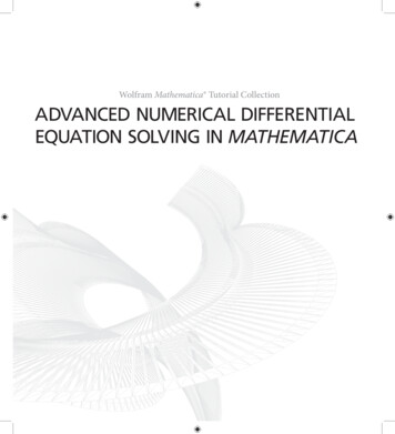
08.06Shooting Methodfor Ordinary Differential EquationsAfter reading this chapter, you should be able to1. learn the shooting method algorithm to solve boundary value problems, and2. apply shooting method to solve boundary value problems.What is the shooting method?Ordinary differential equations are given either with initial conditions or with boundaryconditions. Look at the problem below.υqxLFigure 1 A cantilevered uniformly loaded beam.To find the deflection as a function of location x , due to a uniform load q , theordinary differential equation that needs to be solved isd 2 q L x 2 (1)22 EIdxwhereL is the length of the beam,E is the Young’s modulus of the beam, andI is the second moment of area of the cross-section of the beam.Two conditions are needed to solve the problem, and those are 0 008.06.1
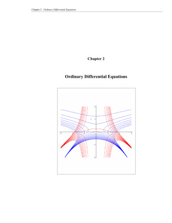
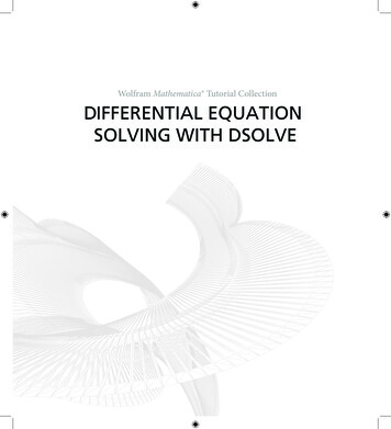
08.06.2Chapter 08.06d 0 0(2a,b)dxas it is a cantilevered beam at x 0 . These conditions are initial conditions as they are givenat an initial point, x 0 , so that we can find the deflection along the length of the beam.Now consider a similar beam problem, where the beam is simply supported on thetwo endsυqxLFigure 2 A simply supported uniformly loaded beam.To find the deflection as a function of x due to the uniform load q , the ordinarydifferential equation that needs to be solved isd 2 qx x L (3)22 EIdxTwo conditions are needed to solve the problem, and those are 0 0 L 0(4a,b)as it is a simply supported beam at x 0 and x L . These conditions are boundaryconditions as they are given at the two boundaries, x 0 and x L .The shooting methodThe shooting method uses the same methods that were used in solving initial value problems.This is done by assuming initial values that would have been given if the ordinary differentialequation were an initial value problem. The boundary value obtained is then compared withthe actual boundary value. Using trial and error or some scientific approach, one tries to getas close to the boundary value as possible. This method is best explained by an example.Take the case of a pressure vessel that is being tested in the laboratory to check itsability to withstand pressure. For a thick pressure vessel of inner radius a and outer radiusb , the differential equation for the radial displacement u of a point along the thickness isgiven byd 2 u 1 du u 0dr 2 r dr r 2(5)Assume that the inner radius a 5" and the outer radius b 8" , and the material of thepressure vessel is ASTM36 steel. The yield strength of this type of steel is 36 ksi. Two straingages that are bonded tangentially at the inner and the outer radius measure the normaltangential strain in the pressure vessel as t / r a 0.00077462
Shooting Method08.06.3 t / r b 0.00038462(6ab)rabFigure 3 Cross-sectional geometry of a pressure vessel.at the maximum needed pressure. Since the radial displacement and tangential strain arerelated simply byu t ,(7)rthenu r a 0.00077462 5 0.0038731' 'ur b 0.00038462 8 0.0030770' 'Starting with the ordinary differential equationd 2u 1 du u 0, u 5 0.0038731, u 8 0.0030770dr 2 r dr r 2Letdu wdrThendw 1u w 2 0dr rrgiving us two first order differential equations asdu w, u 5 0.0038731"drdww u 2 , w 5 not knowndrr rLet us assumedu 5 u 8 u 5 0.00026538w 5 dr8 5Set up the initial value problem.du w f1 r , u , w , u 5 0.0038731"dr(8)(9)(10)(11a,b)
08.06.4Chapter 08.06dww u 2 f 2 r , u, w , w 5 0.00026538drr rUsing Euler’s method,u i 1 u i f1 ri , u i , wi hwi 1 wi f 2 ri , u i , wi hLet us consider 4 segments between the two boundaries, r 5" and r 8" , then8 5h 0.75"4i 0, r0 5, u0 0.0038731", w0 0.00026538u1 u 0 f 1 r0 , u 0 , w0 h 0.0038371 f1 5,0.0038371, 0.00026538 (0.75) 0.0038371 0.00026538 (0.75) 0.0036741"w1 w0 f 2 r0 , u 0 , w0 h 0.00026538 f 2 (5,0.0038731, 0.00026538) 0.75 0.00026538 0.0038371 0.00026538 0.75 552 0.00010938i 1, r1 r0 h 5 0.75 5.75",u1 0.0036741", w1 0.00010940u 2 u1 f1 r1 , u1 , w1 h 0.0036741 f1 5.75,0.0036741, 0.00010938 0.75 0.0036741 0.00010938 (0.75) 0.0035920 ″w2 w1 f 2 r1 , u1 , w1 h 0.00010938 f 2 5.75,0.0036741, 0.00010938 0.75 0.00010938 0.00013015 (0.75) 0.000011769i 2, r2 r1 h 5.75 0.75 6.5"u 2 0.0035920" , w2 0.000011785u 3 u 2 f 1 r2 , u 2 , w2 h 0.0035920 f1 6.5,0.0035920, 0.000011769 0.75 0.0035920 0.000011769 (0.75) 0.0035832"w3 w2 f 2 r2 , u2 , w2 h 0.000011769 f 2 6.5,0.0035920 0.000011769 (0.75)(12a,b)(13a,b)
Shooting Method08.06.5 0.000011769 0.000086829 (0.75) 0.000053352i 3, r3 r2 h 6.50 0.75 7.25"u3 0.0035832", w3 0.000053352u 4 u 3 f1 r3 , u 3 , w3 h 0.0035832 f1 7.25,0.0035832,0.000053352 (0.75) 0.0035832 0.000053352 (0.75) 0.0036232"w4 w3 f 2 r3 , u 3 , w3 h 0.000011785 f 2 7.25,0.0035832, 0.000053352 (0.75) 0.000053352 0.000060811 (0.75) 0.000098961Atr r4 r3 h 7.25 0.75 8"we haveu4 u 8 0.0036232"While the given value of this boundary condition isu4 u 8 0.003070"du 5 . Based on the first assumed value, maybe using twiceLet us assume a new value fordrthe value of initial guess.duu 8 u 5 w 5 2 5 2 2 0.00026538 0.00053076dr8 5Using h 0.75 , and Euler’s method, we getu4 u 8 0.0029665"While the given value of this boundary condition isu4 u 8 0.0030770"Can we use the results obtained from the two previous iterations to get a better estimate ofdu 5 ? One method is to use linear interpolation on thethe assumed initial condition ofdrdu 5 .obtained data for the two assumed values ofdrWithdu 5 0.00026538,drwe obtained
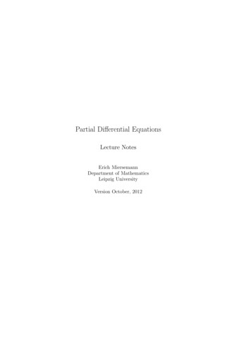
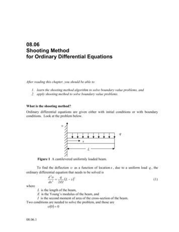
08.06.6Chapter 08.06u 8 0.0036232" , andwithdu 5 0.00053076,drwe obtainedu 8 0.0029665"du 5 knowing that the actual value atso a better starting value ofdru 8 0.00030770" ,we getdu 5 0.00053076 0.00026538 0.0030770 0.0036232 0.00026538 0.0029645 0.0036232dr 0.00048611Using h 0.75" , and repeating the Euler’s method withw 5 0.00048611 ,we getu4 u 8 0.0030769"while the actual given value of this boundary condition isu 8 0.0030770" .In this case, this value coincides with the actual value of u 8 . If that were not the case, onewould continue to use linear interpolation to refine the value of u 4 till one gets close to theactual value of u 8 . Note that the step size and the numerical method used would influencethe accuracy for the obtained values. For the last case, the values are as followsu0 u 5 0.0038731"u1 u 5.75 0.0035085"u2 u 6.50 0.0032858"u3 u 7.25 0.0031518"u 4 u 8.00 0.0030770"See Figure 4 for the comparison of the results with different initial guesses of the slope.Using h 0.75 ″ and Runge-Kutta 4th order method,u1 u 5 0.0038731"u2 u 5.75 0.0035554"u3 u 6.50 0.0033341"u4 u 7.25 0.00317923"u5 u 8 0.0030723"
Shooting Method08.06.74.0E-03du/dr -0.00026538Radial Displacement, u (in)3.8E-033.6E-03Exact3.4E-03du/d r -0.000486113.2E-03du/dr -0.000530763.0E-0356Radial Location, r (in)78Figure 4 Comparison of results with different initial guesses of slopeTable 1 shows the comparison of the results obtained using Euler’s, Runge-Kutta and exactmethods.Table 1 Comparison of Euler and Runge-Kutta results with exact results.rExactEulerRunge-Kutta t (%)(in)(in)(in)(in)55.756.57.2583.8731 10-33.5567 10-33.3366 10-33.1829 10-33.0770 10-33.8731 10-33.5085 10-33.2858 10-33.1518 10-33.0770 10-30.00001.37311.54829.8967 10-11.9500 10-33.8731 10-33.5554 10-33.3341 10-33.1792 10-33.0723 10-3ORDINARY DIFFERENTIAL EQUATIONSTopicShooting methodSummaryTextbook notes on the shooting method for ODE.MajorGeneral EngineeringAuthorsAutar KawLast Revised December 23, 2009Web Sitehttp://numericalmethods.eng.usf.edu t (%)0.00003.5824 10-27.4037 10-21.1612 10-11.5168 10-1
1.9500 10-3 3.8731 10-3 3.5554 10-3 3.3341 10-3 3.1792 10-3 3.0723 10-3 0.0000 3.5824 10-2 7.4037 10-2 1.1612 10-1 1.5168 10-1 ORDINARY DIFFERENTIAL EQUATIONS Topic Shooting method Summary Textbook notes on the shooting method for ODE. Major General Engineering Authors Autar Kaw Last Revised December 23, 2009