Transcription
Journal of Optimization in Industrial Engineering 16 (2014) 83-99Facility Location and Inventory Balancing in a Multi-period Multiechelon Multi-objective Supply Chain: An MOEA ApproachSeyed Habib A. Rahmatia, Abbas Ahmadib,*, Behrooz KarimicaPhD Candidate, Industrial Engineering Department, Amirkabir University of Technology, Tehran, IranbAssistant Professor, Industrial Engineering Department, Amirkabir University of Technology, Tehran, IrancAssociate Professor, Industrial Engineering Department, Amirkabir University of Technology, Tehran, IranReceived 18 September, 2013; Revised 20 November, 2013; Accepted 27 March, 2014AbstractA comprehensive and integrated study of any supply chain (SC) environment is a vital requirement that can create various advantages forthe SC owners. This consideration causes productive managing of the SC through its whole wide components from upstream suppliers todownstream retailers and customers. On this issue, despite many valuable studies reported in the current literature, considerable gaps stillprevail. These gaps include integration and insertion of basic concepts, such as queuing theory, facility location, inventory management, oreven fuzzy theory, as well as other new concepts such as strategic planning, data mining, business intelligence, and information technology.This study seeks to address some of these gaps. To do so, it proposes an integrated four-echelon multi-period multi-objective SC model. Tomake the model closer to the real world problems, it is also composed of inventory and facility location planning, simultaneously. Theproposed model has a mixed integer linear programming (MILP) structure. The objectives of the model are reducing cost and minimizingthe non-fill rate of customer zones demand. The cost reduction part includes cost values of raw material shipping from suppliers to plants,plant location, inventory holding costs in plants, distribution cost from plants to warehouses or distribution centers (DCs), and shippingcosts from DCs to customer zones. Finally, since the literature of SC lacks efficient Pareto-based multi-objective evolutionary algorithms(MOEAs), a new multi-objective version of the biogeography-based optimization algorithm (MOBBO) is introduced to the literature of theSC. The efficiency of the algorithm is proved through its comparison with an existing algorithm called multi-objective harmony search(MOHS).Keywords: Integrated supply chain management, Production-distribution, Facility location problem, inventory balancing, Planningproblem, MOBBO, MOHS.1. Introductionof the distribution centers and logistic warehouse, queuingissues, inventory controlling and balancing. Someresearchers have focused on only one of these items whileothers have considered the combination of two or more ofthem.One of the important combinations in the literature isthe combination of production area of the SC with thedistribution part of it, known as production-distributionproblems. In this class, Jayarman and Pirkul (2001)considered factory, distribution center, and demand areawithin their multi-product deterministic SC. Yilmaz andCagatay (2006) introduced a three-stage strategicplanning for their production-distribution network. In thismodel, which considers one product, multi-suppliers,multi-manufacturers, and multi-distributers, demand isdeterministic and the objective is to minimize cost ofproduction, transportation, and inventory. Some reviewpapers are also presented on this subject (Erenguc etal.,1999, Chen, 2004). Some papers focus on inventoryDifferent definitions have been proposed for supply chain(SC) in the literature. Generally, it is defined as anintegrated system of facilities and activities thatsynchronizes inter-related business functions of materialprocurement, material transformation to intermediates andfinal products and distribution of these products tocustomers (Simchi-Levi, 2000). In other words, the goalof the supply chain management is to integrate suppliers,manufacturers, warehouses, and stores, so that theproduction of the merchandises and their distribution canbe done at the right quantities, to the right locations, andat the right time. The total objective of the system is tominimize system-wide costs while satisfying service levelrequirements of the customers.Since SC covers a vast range of concepts and methods,various issues are evolved as the subjects of the industrialand academic research in SC. Some common issuesinclude supplier selection, production-distributionplanning, transportation and distribution, facility location* Corresponding author Email address: abbas.ahmadi@aut.ac.ir83
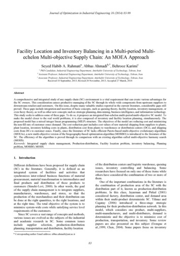
Seyed Habib A. Rahmati et al./ Facility Location and Inventory.subject in their supply chain (Muckstadt and Roundy,1987; Chan et al., 2002; Levi et al., 2005). Inventory hasconsiderable role in the studies of SCs as the main arteryof any supply chain. The basic SC model that considersthis item is generally known as single warehouse multiretailer (SWMR) problem (Muckstadt and Roundy, 1987).Federgruen and Zipkin (1984) studied single period, onewarehouse, multi-retailer problem under uncertaindemands. Roundy (1985) proposed a policy with 98%approach in which the multi-objective is not convertedinto a single objective model. These approaches are morepopular these days (Deb et al., 2001). The number ofthese algorithms is not considerable in the literature of theSC though. Vahdani and Sharif (2013) developed aninexact-fuzzy-stochastic optimization model for a closedloop supply chain network design problem.According to the literature, this research proposes anintegrated model which fills some gaps of the literature.To do so, since, in the literature of SC, specifically earches have studied the shortage permittedassumption, this item is considered in our model.Moreover, some other terms of the inventory issue, as themain artery of any SC model, are included in entory parts of the model. In addition, to make themodel more realistic, it is also encompassed facilitylocation planning. The final structure of this model is as amixed integer linear programming (MILP) problem.Furthermore, since the literature lacks efficient Paretobased multi-objective evolutionary algorithms (MOEAs),a new multi-objective version of the biogeography-basedoptimization algorithm (MOBBO) is introduced to theliterature of the SC. Finally, this algorithm is comparedwith an existing algorithm called MOHS (Rahmati et al.2013). The results are also evaluated through differentstatistical and non-statistical tests, tables, and figures.The paper is organized as follow. The developedintegrated model is described in section 2. This sectionincludes problem definition including all parts of themodel ranging from assumptions and indices to objectivefunctions and constraints. Section 3 presents the requiredconcepts and operators of the proposed MOEA. Section 4,through different computational experiments, provesefficiency of the proposed algorithms. Section 5concludes the paper and presents the future works.O(nlogn)effectiveness intime for analyzing a problemwhich permits no shortage or backlogging. Chan andKumar (2009 a, b) investigated a manufacturingenvironment that included warehouse-scheduling problemin a manufacturing environment. Poon et al. (2009)studied order picking operations in warehouses. Anotherimportant issue, which is inserted into SC models, isfacility location. Javid and Azad (2010) solved anintegrated model of facility location, capacity, inventory,and routing. Bidhandi et al. (2009) developed a mixedlinear integer programming problem of multi-commoditysupply chain. They solved their problem usingdecomposition methods. Rappold and Van Roo (2009)studied two-echelon supply chain, which combinedfacility location, inventory allocation, and capacityinvestment.Among the presented studies, most of the researchesare single objective (Williams 1981, Gen and Syarif,2005; Tsiakis and Papageorgiou, 2008). Further, somestudies focus on multi-objective problems in the SC areas.This class is more realistic, because most of the real worldproblems, specifically in the complex environment of theSC problems, cope with several goals. In this class,Altiparmak et al. (2006) developed a multi-objectiveshortage forbidden model that investigated networkstructure of manufacturers and customer area. Theirmodel tried to minimize costs, deliver time and balance ofthe capacity of the factories. Jolai et al. (2011) proposed alinear multi-objective production-distribution model.Their model considered a SC with multi-products, levels,and periods. However, they changed their model into asingle objective model in their solving approach. Sadeghiet al. (2011) developed a single-vendor single-retailer in amulti-product supply chain. Aliakbari and Seifbarghy(2011) introduced a social responsible supplier selectionmodel. Songsong and Lazaros (2012) also studied a multiobjective production-distribution model. Their modelconsidered a universal SC with three objectives of costs,response, and service level. Taherkhani and Seifbarghy(2012) determined the material flows in a multi-echelonassembly supply chain. Shankar et al. (2013), in theirmulti-objective production-distribution, proposed singleproduct four-echelon supply chain architecture. They alsoconsidered facility location planning in their problem.However, they did not consider the inventory issue intheir integrated model. They solved their model via amulti-objective hybrid particle swarm optimization(MOHPSO) algorithm. Their approach is a Pareto-based2. Problem DefinitionIn this section, the integrated SC model is described.The proposed SC model of this research is a multiechelon multi-period model which encompasses inventoryand facility location planning simultaneously. Theinventory part of the model includes four-echelon multiperiod inventory cost as the objective function andinventory balancing among different echelon withindifferent periods. The structure of the proposed model isas MINLP. Figure 1 illustrates a simple structure of thismodel, schematically. The rest of this section defines therequired definitions and notations and then formulates themain model in different subsections.2.1. Notationsl: Number of suppliers (h 1, 2, , l)n: Number of potential plant locations (i 1, 2, , n)84
Journal of Optimization in Industrial Engineering 16 (2014) 83-99t: Number of warehouse (DC) locations (e 1, 2, ,ICcik : Inventory holding cost of component c in plant i attime period k c : Consume coefficient of component ct)m: Number of customer zones (markets) or demandpoints (j 1, 2, , m)p: Number of components (c 1, 2, , p)s: Number of time periods (k 1, 2, , s)2.3. Decision variables2.2. ParametersYi : 1, if plant i is open, 0 otherwiseD jk : Average demand from markets j at time period kY 'e : 1, if warehouse e is open, 0 otherwiseX hcik : Quantity of component c shipped from supplier hto plant i at time period kKik : Potential capacity of plant i at time period kKek : Potential capacity of warehouse e at time period kSchk : Supply capacity by supplier h from component c atX 'ejk : Quantity shipped from warehouse e to customerzone j at time period ktime period kFi : Annual fixed cost of keeping open of plant iX "iek : Quantity shipped from plant i to warehouse e attime period kI cik : Inventory quantity of component c in plant i at timeperiod kFe : Annual fixed cost of keeping open of warehouse eChcik : Cost of making and shipping a components c fromsupply source h to plant i at time period kCiek : Cost of producing and shipping one unit from planti to warehouse e at time period kCejk : Cost of throughput and shipping one unit fromI 'ek : Inventory quantity in warehouse e at time period kI "ik : Inventory quantity in plant i at time period k2.4. The main modelwarehouse e to customer j at time period kICik : Inventory holding cost of one unit in plant i at timeperiod kICek : Inventory holding cost of one unit in warehouse eat time period knMin Z1 t fi Yi i 1t mf e Y 'en e 1 Cejk e 1 j 1 k 1nsmsnts Chcik X hcik Ciek X "ieki 1 e 1 k 1ns ICcik I cik c 1 i 1 k 1tpi 1 h 1 c 1 k 1psX 'ejklThis subsection presents the main proposed model asfollows.tICik I "iki 1 k 1 (1)s' ICek I eke 1 k 1s X 'ejkMin Z 2 1 e 1 j 1 k 1m s(2) D jkj 1 k 1s.t.n X hcik Schk h 1, 2, ., l , c 1, 2, ., p, k 1, 2, ., s(3)i 1t X 'ejk D jk j 1, 2, ., m, k 1, 2, ., s(4)e 1t X "iek KikYi i 1, 2, ., n, k 1, 2, ., se 185(5)
Seyed Habib A. Rahmati et al./ Facility Location and Inventory.m X 'ejk Kek Y 'e e 1, 2, ., t , k 1, 2, ., s(6)j 1lt X hcik X "iek 0h 1ne 1mi 1j 1 i 1, 2, ., n, c 1, 2, ., p, k 1, 2, ., s X "iek X 'ejk 0lI cik I cik 1 e 1, 2, ., t , k 1, 2, ., s(7)(8)tX hcik h 1 c X 'iek c 1, 2, ., p, i 1, 2, ., n, k 1, 2, ., s(9)e 1I "ik I "ik 1 Kik t X "iek i 1, 2, ., n, k 1, 2, ., s(10)e 1I 'ek I 'ek 1 n i 1X "iek m X 'ejk e 1, 2, ., t , k 1, 2, ., s(11)j 1X hcik , X "iek , X 'ejk , I ick , I "ik , I 'ek 0Yi , Y 'e 0,1 (12)I ci 0 I "i 0 , I 'e0 0nIn this model, Eq.1 models the first objective function,which minimizes the total cost in supply chain. Total costincludes raw material shipping from suppliers to plants,plant location, inventory holding costs in plants,distribution cost from plants to warehouses or distributioncenters (DCs), throughput and shipping costs from DCs tocustomer zones.The objective function (2) is minimizing the non-filledrate of customer zones demand.Equation (3) ensures that the total quantity shipped from asupplier at each period cannot exceed the supply capacity.Equation (4) indicates that the demand at customer zoneshould be satisfied to the maximum extend.Equation (5) shows that no plant can supply more than itscapacity if the plant is opened.The Equation in (6) represents that no warehouse cansupply more than its capacity if the warehouse is opened.Equation (7) ensures that the quantity shipped out of aplant cannot exceed the component quantity received.Consequently, equation (8) ensures that the quantityshipped out of a warehouse cannot exceed the quantityreceived.Equations (9) and (10) represent the inventory balanceconstraint in plant.Equation (11) is the inventory balance equation for DC.For example, in this equation, inventory of one unit inperiod k ( X "iek ) minus amount of one unit shippedi 1from DC e to customer zones (CZs), at time periodm X 'ejk ) . Finally, constraint (12) shows positive andk(j 1binary variables.Figure 1 illustrates the diagram of this supply chainschematically.3. Solving MethodologyAs mentioned earlier, the developed model of thisresearch has MINLP structure. It is proved that simplermodel than this model are NP-Hard (Shankar et al., 2013).Therefore, a meta-heuristic approach is proposed tosolved the problem. This approach introduces MOBBOalgorithm to the SC area. This algorithm is a MOEAbased on biogeography optimization (BBO) algorithm asthe single objective version. BBO is a population-basedoptimization algorithm (Simon, 2008). Therefore, it hasdifferent similarities with other existing population-basedalgorithms like genetic algorithm (GA) or particle swarmoptimization (PSO). Generally, in this type of algorithmwe have a set of individuals that is called population. Theindividual in this algorithm is called habitat or island. Anyfeature of the individual (like gene in GA) here is knownas a SIV. The fitness value of the individuals here ismeasured by high suitability index (HSI). However, it hassome distinctive differences with the existing populationbased algorithms. For instance, in this algorithm, instead'warehouse e and at time period k ( I ek ) is equal to theinventory at one time unit of previous period ( I 'ek 1 ) plusamount of one unit shipped from plants to DC e at time86
Journal of Optimization in Industrial Engineering 16 (2014) 83-99of fitness value migration rates are used to guide thealgorithm.Fig. 1. A four layers diagram of the proposed supply chainActually, in biogeography science migration is dividedinto two different performances of the species, includingemigration and immigration. For each of theseperformances, a specific rate is also considered calledfront, is the goal of MOEA. Improvement in multiobjective environment has two signs, including (1)improving the convergence to the optimal front, or (2)improving the diversity of the existing solutions of aPareto front. Therefore, it is expected that the finalobtained Pareto front of an MOEA has an appropriateconvergence and diversity. To evaluate these two types ofthe improvement in a MOEA, different types of measurescan be used, some of which will be introduced and used inthe next section.emigration rate ( j ) and immigration rate ( i ).Emigration rate determines how likely a species(emigrating species) shares its features with other species(immigrating species). Likewise, immigration ratedetermines how likely a species (immigrating species)accepts features from other species (emigrating species).In a relation with HSI, it can be expected that featuresmigrate from high-HSI habitats (emigrating habitat) tolow-HSI habitats (immigrating habitat). Therefore, byusing migration rates, the aim of the BBO is to guide theoptimization process in a way that the HSI is maximized(Rahmati and Zandieh, 2012).Now, before explaining the operators of this algorithm,since this paper is going to introduce multi-objectiveversion of the BBO, the fundamental principles anddefinitions of MOAs are introduced.3.2. Representation, Initialization and decoding scheme ofthe habitatsIn MOBBO, like any other population-based algorithm,the optimization process starts with initializing the initialpopulation. The proposed habitat is composed of threerows by which some constraints are satisfied based on thevalues of decision variables. The first row represents thatfacilities such as plant and warehouse are open or close inbinary representation. The second row includes thequantity shipped through suppliers, plants, DCs and CZs.The third row indicates the amount of inventory level inplants and warehouses. The general form of a habitatstructure is represented in Figure 2.In the first row of this habitat, potential location of plantsand warehouses are coded as binary variables. Theamount of shipped components and one unit of productare calculated according to supply capacity of suppliers,plants, DCs and demand of markets at each time period insecond row of solution. For example, quantity shippedfrom a plant to DCs at time period k is less than plantcapacity. In addition, this amount should be less equalthan the component amount shipped from suppliers toplant.3.1. Multi-objective principlesInamulti-objectiveproblemsubject f ( x ) f1 ( x ),., f m ( x ) gi ( x ) 0, i 1,2,., c, x X , dominate solution b ( a , b X )solutionliketo acanif following twoconditions are held simultaneously: 1) f i ( a ) f i (b ), i 1, 2, ., m 2) i {1, 2, ., m}: f i ( a ) f i (b )Now, in different iterations of the MOEA, a set ofsolutions that cannot dominate each other is known asPareto solutions set or Pareto front. Improving this Paretofront, during different iterations to achieve Pareto optimal87
Seyed Habib A. Rahmati et al./ Facility Location and Inventory.Fig. 2. The habitat structure of the MOBBOIn the third row of habitat, inventory levels in plants andwarehouses are decoded considering the second row ofthe habitat. For example, the amount of one unit that isdelivered to DC must be equal to the amount of one unitthat leaves from and is stored in this DC. In order toprevent the negative and infeasible solutions in this part,until the inventory quantity is negative, a random numberbetween zero and one is generated. If the value of thisnumber is less than a predetermined value, a plant isselected randomly, and the amount of shipped items isequal to the minimum total of this value with inventorydeficit and plant capacity to ship. Otherwise, a customerzone (CZ) is selected randomly and the amount of shippedfrom DC is equal to maximum difference of this amountwith inventory deficit and zero value to generate feasiblesolutions of both states.for selecting the emigrating habitat. To do so, aftercalculating of the CDs and FNDSs, if a specific habitatneeds to be immigrated, two habitats are selectedrandomly. Then, if they are from different ranks (ordifferent front), the one with lower rank is selected;otherwise, the one with higher CD is selected as theemigrating habitat. A scheme of this selection strategy canbe seen in Figure 7.Now, to implement migration operator, it is necessary tocalculate i and j . The method of this calculation is thethird (and the last) main factor that distinguishes MOBBOfrom its single version. After sorting the population,immigration rate i andemigration rate j can beevaluated as Eq.13 and Eq. 14, respectively. In theseequations, ki represents rank of ith habitat after sortingall habitats according to multi-objective strategy and nrepresents size of the population. Of course, it should be3.3. Sorting strategyThis operator is the first main factor that distinguishesMOBBO from its single version. In this part, afterdecoding the habitats and calculating their HSIs, insteadof sorting the population according to the HSI’s values, amulti-objective strategy is used. This strategy is proposedby Deb et al. (2000). In this strategy, an operator calledFNDS is used for assigning ranks to individuals of thepopulation due to domination concept. Then, anotheroperator called CD is used to estimate density of solutionswhich are laid surrounding a particular solution in thesame rank. Now, according to these two operators thepopulation is sorted. To do so, in the case of the differentranks (or the individuals from different fronts), the onewith lower rank is better. However, if the ranks are thesame, the one with higher CD is preferred.mentioned that, ki ranging from 1 to n and the highervalues are of more interest.k i I (1 i )nki i E ( )n(13)(14)The inverse relation between these two rates is shown inFigure 3. In this figure, E and I, represents maximumnumber of the migration rates and are usually set at zero,and Si denotes the state of the species amount. Accordingto what was mentioned and this figure, by increasing ofthe number of species (or going for a more suitablehabitat), the immigration rate is decreasing and theemigration rate is increasing. It means that the features ina more suitable habitat with miscellaneous species aremore likely to be emigrated rather than to be immigrated.This is the main concept of the migration.3.4. Selection strategy and migration operatorThis operator is the second main factor that distinguishesMOBBO from its single objective version. In thisselection strategy, a binary tournament selection is used88
Journal of Optimization in Industrial Engineering 16 (2014) 83-99perform migration operator, the structure introduced forthe single objective BBO is used. The Uniformneighborhood structure is used for conducting themigration as Figure 4. In this figure, H represents habitatand n denotes number of the SIVs of each habitat.To show how Uniform migration works, a scheme isplotted in Figure 5. In this structure, the immigratinghabitat accept features from sharing or emigrating habitatfor those cells that their random vector numbers (Rand is0 or 1) is 1.3.5. Mutation operatorsFig. 3. The variation of migration rates toward number of the species(Simon, 2008)In this research, for mutation structure Mask operator isimplemented. The scheme of this operator is illustrated inFigure 5.Figure 3 summarizes the concepts that were proposed inthis sub section to do a quite migration process.According to this figure, it is clear that a good habitat(with low i ) is less likely to be immigrated, while as, apoor habitat (with high i ) is so likely to be. Finally, toFig. 4. The migration operator and the selection strategyFig. 5. Uniform migration operator schemeFig. 6. Mask mutation operator schemeIn this figure, a Mask vector is generated randomly withthe number from the interval [0,1]. Now, for those cells ofthe Mask vector, which have the values less than 0.5, thehabitat is mutated. For conducting this mutation, thementioned cell is regenerated and its value is assignedrandomly.89
Seyed Habib A. Rahmati et al./ Facility Location and Inventory.3.6. The MOBBO’s optimization process3.7 The MOHSThe evolution process of the MOBBO is illustratedschematically in Figure 7. This process is started byAs mentioned above, MOBBO is compared with theMOHS from the literature (Rahmati, 2013). MOHS is aPareto-based multi-objective version of the singleobjective harmony search (HS) algorithm, which isreinforced by the same operators as the ones implementedin this study to get a multi-objective. This algorithmmimics the improvising process of musicians. In HS,three different operators are used, including harmonymemory operator, pitching operator, and random operator.The more elaborate description of this algorithm is foundin Rahmati et al. (2013). However, it is required tomention that for the pitching operator of the MOHS inthis study, a structure just like what explained for themutation of the MOBBO is used.initializing the initial population of the habitat Rt . Then,BBO’s operators, including migration and mutation, areRt to create the new population Qt .The blending of Pt and Qt creates Rt . In this step,habitats of Rt are sorted in several fronts by means of theimplemented onexplained strategy in sub section 3.3. Now, to createPt 1 , while the capacity ofis not exceeded, the fronts are added to Pt 1 ,population of the next iterationaccording to increasing order of their ranks. But, whenwithout a front, Pt 1 has fewer members than population4. Computational Resultssize and with it, Pt 1 has more members than populationsize, the habitats must be selected partially to reach thepredetermined population size. In this situation, thehabitats of the front are sorted in decreasing order of theirCDs, and the habitats of next iteration are chosen from topof the front.In fact, the most differentiation of the MOBBO with theNSGAII (Deb et al., 2000) is their evolution operators. Inother words, the searching heart of the NSGAII is GA, butthe searching heart of MOBBO is BBO. In other terms,instead of some simple differences, they guide the multiobjective process similarity. The pseudo code of theMOBBO is also presented in Figure 8. In this figure, thesearching heart of the MOBBO, which is BBO, isseparated in the middle of the pseudo code.In this section, to assess the developed model and theproposed algorithm, first some test problems aregenerated. Then, the algorithms are compared based onthe whole generated test problems. This comparison ismade through utilizing different types of the statisticaland non-statistical tests and various explanatoryillustrations.4.1. Test problem generatingIn the model study, the parameters are generated as Table1. In this table, U(1000,1500) represents a randomnumber generated in the intervaluniform distribution.Fig. 7. Evolution process of the MOBBO90(1000,1500) from
Journal of Optimization in Industrial Engineering 16 (2014) 83-99Fig. 8. The pseudo code of MOBBOTable1Input data of the modelParameterDistribution functionParameterDistribution functionD )ICcikICikICek cU(5,10)U(2000,8000)U(30,50)U(40,70)Then, to test the generated model, 14 test problems werecreated via the information presented in Table 2. In thistable, the factors that make a distinctive problem arenumber of suppliers (l), plant location (n), DCs (T), andU(8,12)U(10,15)U(0,1)CZs (m). Moreover, 5 raw material types and at 3 timeperiods are considered.91
Seyed Habib A. Rahmati et al./ Facility Location and Inventory.4.2. Outputs of the algorithms on the generated testproblems4.2.1. Multi-objective metric descriptionGenerally, two main features are considered to evaluatethe performance of a MOEA.1) The first feature assesses whether the final Paretofront of the algorithm is converged to the Paretooptimal front or not.2) The second feature evaluates the diversification ofthe set of solutions of the Pareto front.In this subsection, after defining some requireddefinitions, the outputs of the algorithms are evaluated.The definitions include the implemented metrics and thetests used.Table 2Generated test problemsTest 77791012151820202020Table 3Utilized performance measuresMetricT34679121215182022252525Metric calculationMetric brief descriptionIt is used to evaluate the spread of thefront.mDiversity(Zitzler, 1999) ( ) ( m ax fD i 1:niji m in f j )M56710121517202530354048702i 1:nj 1S Spacing(Schott, 1995) ( )1n 1Simultaneous metric (SM)(Rahmati et al., 2013) ( )2* (d i d ) d i i 1M ID k f j f j d j 1ciNOSi 1di n mwhere c i (fj 1SM MIDDNumber of the non-dominatedsolutions in final Pareto( NOS ) (Rahmati et al.,n ik n Λ k iIt is used to measure the uniformity of thesolutions within a front. mminMean ideal distance (MID)(Rahmati et al., 2012) ( )nij)2It is used to measure the closeness ofsolutions in a Pareto front with an idealpoint which is usually considered as (0, 0).This metric considers the two features ofthe MOEAs simultaneously.Measures number of the Pareto solutions.-2012) ( )di : denotes the space between two neighbor solutions n :denotes the number of the existing solutions in the Paretofrontsm: denotes the number of the objective functionsf ji : denotes the jth objective funct
The proposed SC model of this research is a multi-echelon multi-period model which encompasses inventory and facility location planning simultaneously. The inventory part of the model includes four-echelon multi-period inventory cost as the objective function and inventory balancing among different echelon within different periods.