Transcription
Fast Algorithms for Mining Association RulesRakesh AgrawalRamakrishnan Srikant IBM Almaden Research Center650 Harry Road, San Jose, CA 95120AbstractWe consider the problem of discovering association rulesbetween items in a large database of sales transactions.We present two new algorithms for solving this problemthat are fundamentally di erent from the known algorithms. Empirical evaluation shows that these algorithmsoutperform the known algorithms by factors ranging fromthree for small problems to more than an order of magnitude for large problems. We also show how the bestfeatures of the two proposed algorithms can be combinedinto a hybrid algorithm, called AprioriHybrid. Scale-upexperiments show that AprioriHybrid scales linearly withthe number of transactions. AprioriHybrid also has excellent scale-up properties with respect to the transactionsize and the number of items in the database.1 IntroductionProgress in bar-code technology has made it possible for retail organizations to collect and store massive amounts of sales data, referred to as the basketdata. A record in such data typically consists of thetransaction date and the items bought in the transaction. Successful organizations view such databasesas important pieces of the marketing infrastructure.They are interested in instituting information-drivenmarketing processes, managed by database technology, that enable marketers to develop and implementcustomized marketing programs and strategies [6].The problem of mining association rules over basketdata was introduced in [4]. An example of such arule might be that 98% of customers that purchase Visiting from the Department of Computer Science, University of Wisconsin, Madison.Permission to copy without fee all or part of this materialis granted provided that the copies are not made or distributedfor direct commercial advantage, the VLDB copyright noticeand the title of the publication and its date appear, and noticeis given that copying is by permission of the Very Large DataBase Endowment. To copy otherwise, or to republish, requiresa fee and/or special permission from the Endowment.Proceedings of the 20th VLDB ConferenceSantiago, Chile, 1994tires and auto accessories also get automotive servicesdone. Finding all such rules is valuable for crossmarketing and attached mailing applications. Otherapplications include catalog design, add-on sales,store layout, and customer segmentation based onbuying patterns. The databases involved in theseapplications are very large. It is imperative, therefore,to have fast algorithms for this task.The following is a formal statement of the problem[4]: Let I fi1 ; i2; . . .; im g be a set of literals,called items. Let D be a set of transactions, whereeach transaction T is a set of items such that T I . Associated with each transaction is a uniqueidenti er, called its TID. We say that a transactionT contains X, a set of some items in I , if X T .An association rule is an implication of the formX ) Y , where X I , Y I , and X \ Y ;.The rule X ) Y holds in the transaction set D withcon dence c if c% of transactions in D that containX also contain Y . The rule X ) Y has support sin the transaction set D if s% of transactions in Dcontain X [ Y . Our rules are somewhat more generalthan in [4] in that we allow a consequent to have morethan one item.Given a set of transactions D, the problem of mining association rules is to generate all association rulesthat have support and con dence greater than theuser-speci ed minimum support (called minsup ) andminimum con dence (called minconf ) respectively.Our discussion is neutral with respect to the representation of D. For example, D could be a data le,a relational table, or the result of a relational expression.An algorithm for nding all association rules,henceforth referred to as the AIS algorithm, was presented in [4]. Another algorithm for this task, calledthe SETM algorithm, has been proposed in [13]. Inthis paper, we present two new algorithms, Aprioriand AprioriTid, that di er fundamentally from thesealgorithms. We present experimental results showing
that the proposed algorithms always outperform theearlier algorithms. The performance gap is shown toincrease with problem size, and ranges from a factor of three for small problems to more than an order of magnitude for large problems. We then discuss how the best features of Apriori and AprioriTid can be combined into a hybrid algorithm, calledAprioriHybrid. Experiments show that the AprioriHybrid has excellent scale-up properties, opening upthe feasibility of mining association rules over verylarge databases.The problem of nding association rules falls withinthe purview of database mining [3] [12], also calledknowledge discovery in databases [21]. Related, butnot directly applicable, work includes the inductionof classi cation rules [8] [11] [22], discovery of causalrules [19], learning of logical de nitions [18], ttingof functions to data [15], and clustering [9] [10]. Theclosest work in the machine learning literature is theKID3 algorithm presented in [20]. If used for ndingall association rules, this algorithm will make as manypasses over the data as the number of combinationsof items in the antecedent, which is exponentiallylarge. Related work in the database literature isthe work on inferring functional dependencies fromdata [16]. Functional dependencies are rules requiringstrict satisfaction. Consequently, having determineda dependency X ! A, the algorithms in [16] considerany other dependency of the form X Y ! Aredundant and do not generate it. The associationrules we consider are probabilistic in nature. Thepresence of a rule X ! A does not necessarily meanthat X Y ! A also holds because the latter maynot have minimumsupport. Similarly, the presence ofrules X ! Y and Y ! Z does not necessarily meanthat X ! Z holds because the latter may not haveminimum con dence.There has been work on quantifying the \usefulness" or \interestingness" of a rule [20]. What is useful or interesting is often application-dependent. Theneed for a human in the loop and providing tools toallow human guidance of the rule discovery processhas been articulated, for example, in [7] [14]. We donot discuss these issues in this paper, except to pointout that these are necessary features of a rule discovery system that may use our algorithms as the engineof the discovery process.1.1 Problem Decomposition and PaperOrganizationThe problem of discovering all association rules canbe decomposed into two subproblems [4]:1. Find all sets of items (itemsets) that have transaction support above minimum support. The supportfor an itemset is the number of transactions thatcontain the itemset. Itemsets with minimum support are called large itemsets, and all others smallitemsets. In Section 2, we give new algorithms,Apriori and AprioriTid, for solving this problem.2. Use the large itemsets to generate the desired rules.Here is a straightforward algorithm for this task.For every large itemset l, nd all non-empty subsetsof l. For every such subset a, output a rule ofthe form a ) (l , a) if the ratio of support(l)to support(a) is at least minconf. We need toconsider all subsets of l to generate rules withmultiple consequents. Due to lack of space, we donot discuss this subproblem further, but refer thereader to [5] for a fast algorithm.In Section 3, we show the relative performanceof the proposed Apriori and AprioriTid algorithmsagainst the AIS [4] and SETM [13] algorithms.To make the paper self-contained, we include anoverview of the AIS and SETM algorithms in thissection. We also describe how the Apriori andAprioriTid algorithms can be combined into a hybridalgorithm, AprioriHybrid, and demonstrate the scaleup properties of this algorithm. We conclude bypointing out some related open problems in Section 4.2 Discovering Large ItemsetsAlgorithms for discovering large itemsets make multiple passes over the data. In the rst pass, we countthe support of individual items and determine whichof them are large, i.e. have minimumsupport. In eachsubsequent pass, we start with a seed set of itemsetsfound to be large in the previous pass. We use thisseed set for generating new potentially large itemsets,called candidate itemsets, and count the actual support for these candidate itemsets during the pass overthe data. At the end of the pass, we determine whichof the candidate itemsets are actually large, and theybecome the seed for the next pass. This process continues until no new large itemsets are found.The Apriori and AprioriTid algorithms we proposedi er fundamentally from the AIS [4] and SETM [13]algorithms in terms of which candidate itemsets arecounted in a pass and in the way that those candidatesare generated. In both the AIS and SETM algorithms,candidate itemsets are generated on-the- y during thepass as data is being read. Speci cally, after readinga transaction, it is determined which of the itemsetsfound large in the previous pass are present in thetransaction. New candidate itemsets are generated byextending these large itemsets with other items in thetransaction. However, as we will see, the disadvantage
is that this results in unnecessarily generating andcounting too many candidate itemsets that turn outto be small.The Apriori and AprioriTid algorithms generatethe candidate itemsets to be counted in a pass byusing only the itemsets found large in the previouspass { without considering the transactions in thedatabase. The basic intuition is that any subsetof a large itemset must be large. Therefore, thecandidate itemsets having k items can be generatedby joining large itemsets having k , 1 items, anddeleting those that contain any subset that is notlarge. This procedure results in generation of a muchsmaller number of candidate itemsets.The AprioriTid algorithm has the additional property that the database is not used at all for counting the support of candidate itemsets after the rstpass. Rather, an encoding of the candidate itemsetsused in the previous pass is employed for this purpose.In later passes, the size of this encoding can becomemuch smaller than the database, thus saving muchreading e ort. We will explain these points in moredetail when we describe the algorithms.Notation We assume that items in each transactionare kept sorted in their lexicographic order. It isstraightforward to adapt these algorithms to the casewhere the database D is kept normalized and eachdatabase record is a TID, item pair, where TID isthe identi er of the corresponding transaction.We call the number of items in an itemset its size,and call an itemset of size k a k-itemset. Items withinan itemset are kept in lexicographic order. We usethe notation c[1] c[2] . . . c[k] to represent a kitemset c consisting of items c[1]; c[2]; . .c[k], wherec[1] c[2] . . . c[k]. If c X Y and Yis an m-itemset, we also call Y an m-extension ofX. Associated with each itemset is a count eld tostore the support for this itemset. The count eld isinitialized to zero when the itemset is rst created.We summarize in Table 1 the notation used in thealgorithms. The set C k is used by AprioriTid and willbe further discussed when we describe this algorithm.2.1 Algorithm AprioriFigure 1 gives the Apriori algorithm. The rst passof the algorithm simply counts item occurrences todetermine the large 1-itemsets. A subsequent pass,say pass k, consists of two phases. First, the largeitemsets Lk,1 found in the (k , 1)th pass are used togenerate the candidate itemsets Ck , using the apriorigen function described in Section 2.1.1. Next, thedatabase is scanned and the support of candidates inCk is counted. For fast counting, we need to e cientlydetermine the candidates in Ck that are contained in aTable 1: Notationk-itemset An itemset having k items.Set of large k-itemsetsLk(those with minimum support).Each member of this set has two elds:i) itemset and ii) support count.Set of candidate k-itemsetsCk(potentially large itemsets).Each member of this set has two elds:i) itemset and ii) support count.Set of candidate k-itemsets when the TIDsCkof the generating transactions are keptassociated with the candidates.given transaction t. Section 2.1.2 describes the subsetfunction used for this purpose. See [5] for a discussionof bu er management.1) L1 flarge 1-itemsetsg;2) for ( k 2; Lk,1 6 ;; k ) do begin3) Ck apriori-gen(Lk,1 ); // New candidates4) forall transactions t 2 D do begin5)Ct subset(Ck , t); // Candidates contained in t6)forall candidates c 2 Ct do7)c:count ;8) end9) Lk fc 2 Ck j c:count minsup g10) end11) Answer k Lk ;SFigure 1: Algorithm Apriori2.1.1 Apriori Candidate GenerationThe apriori-gen function takes as argument Lk,1,the set of all large (k , 1)-itemsets. It returns asuperset of the set of all large k-itemsets. Thefunction works as follows. 1 First, in the join step,we join Lk,1 with Lk,1:insert into kselect .item1 , .item2 , ., .itemk,1 , .itemk,1from k,1 , k,1where .item1 .item1 , . . ., .itemk,2 .itemk,2 ,CpLpppLpqqq.itemk,1 q.itemk,1 ;pqpNext, in the prune step, we delete all itemsets c 2 Cksuch that some (k , 1)-subset of c is not in Lk,1:1 Concurrent to our work, the following two-step candidategeneration procedure has been proposed in [17]:00j0 2 k,1 j \ 0 j , 2gk f [0k f 2 k j contains members of k ,1 gThese two steps are similar to our join and prune stepsrespectively. However, in general, step 1 would produce asuperset of the candidates produced by our join step.CXXX; XCXCXL; XkXkL
forall itemsets 2 k doforall ( , 1)-subsets of doif ( 62 k,1 ) thendelete from k ;cCksscLcCExample Let L3 be ff1 2 3g, f1 2 4g, f1 3 4g, f13 5g, f2 3 4gg. After the join step, C4 will be ff1 2 34g, f1 3 4 5g g. The prune step will delete the itemsetf1 3 4 5g because the itemset f1 4 5g is not in L3 .We will then be left with only f1 2 3 4g in C4.Contrast this candidate generation with the oneused in the AIS and SETM algorithms. In pass kof these algorithms, a database transaction t is readand it is determined which of the large itemsets inLk,1 are present in t. Each of these large itemsetsl is then extended with all those large items thatare present in t and occur later in the lexicographicordering than any of the items in l. Continuing withthe previous example, consider a transaction f1 23 4 5g. In the fourth pass, AIS and SETM willgenerate two candidates, f1 2 3 4g and f1 2 3 5g,by extending the large itemset f1 2 3g. Similarly, anadditional three candidate itemsets will be generatedby extending the other large itemsets in L3 , leadingto a total of 5 candidates for consideration in thefourth pass. Apriori, on the other hand, generatesand counts only one itemset, f1 3 4 5g, because itconcludes a priori that the other combinations cannotpossibly have minimum support.Correctness We need to show that Ck Lk .Clearly, any subset of a large itemset must alsohave minimum support. Hence, if we extended eachitemset in Lk,1 with all possible items and thendeleted all those whose (k , 1)-subsets were not inLk,1, we would be left with a superset of the itemsetsin Lk .The join is equivalent to extending Lk,1 with eachitem in the database and then deleting those itemsetsfor which the (k ,1)-itemset obtained by deleting the(k,1)th item is not in Lk,1 . The condition p.itemk,1 q.itemk,1 simply ensures that no duplicates aregenerated. Thus, after the join step, Ck Lk . Bysimilar reasoning, the prune step, where we deletefrom Ck all itemsets whose (k , 1)-subsets are not inLk,1, also does not delete any itemset that could bein Lk .Variation: Counting Candidates of MultipleSizes in One Pass Rather than counting onlycandidates of size k in the kth pass, we can alsocount the candidates Ck0 1, where Ck0 1 is generatedfrom Ck , etc. Note that Ck0 1 Ck 1 since Ck 1 isgenerated from Lk . This variation can pay o in thelater passes when the cost of counting and keeping inmemory additional Ck0 1 , Ck 1 candidates becomesless than the cost of scanning the database.2.1.2 Subset FunctionCandidate itemsets Ck are stored in a hash-tree. Anode of the hash-tree either contains a list of itemsets(a leaf node) or a hash table (an interior node). In aninterior node, each bucket of the hash table points toanother node. The root of the hash-tree is de ned tobe at depth 1. An interior node at depth d points tonodes at depth d 1. Itemsets are stored in the leaves.When we add an itemset c, we start from the root andgo down the tree until we reach a leaf. At an interiornode at depth d, we decide which branch to followby applying a hash function to the dth item of theitemset. All nodes are initially created as leaf nodes.When the number of itemsets in a leaf node exceedsa speci ed threshold, the leaf node is converted to aninterior node.Starting from the root node, the subset functionnds all the candidates contained in a transactiont as follows. If we are at a leaf, we nd which ofthe itemsets in the leaf are contained in t and addreferences to them to the answer set. If we are at aninterior node and we have reached it by hashing theitem i, we hash on each item that comes after i in tand recursively apply this procedure to the node inthe corresponding bucket. For the root node, we hashon every item in t.To see why the subset function returns the desiredset of references, consider what happens at the rootnode. For any itemset c contained in transaction t, therst item of c must be in t. At the root, by hashing onevery item in t, we ensure that we only ignore itemsetsthat start with an item not in t. Similar argumentsapply at lower depths. The only additional factor isthat, since the items in any itemset are ordered, if wereach the current node by hashing the item i, we onlyneed to consider the items in t that occur after i.2.2 Algorithm AprioriTidThe AprioriTid algorithm, shown in Figure 2, alsouses the apriori-gen function (given in Section 2.1.1)to determine the candidate itemsets before the passbegins. The interesting feature of this algorithm isthat the database D is not used for counting supportafter the rst pass. Rather, the set C k is usedfor this purpose. Each member of the set C k isof the form TID; fXk g , where each Xk is apotentially large k-itemset present in the transactionwith identi er TID. For k 1, C 1 corresponds tothe database D, although conceptually each item iis replaced by the itemset fig. For k 1, C k isgenerated by the algorithm (step 10). The member
of C k corresponding to transaction t is t:TID,fc 2 Ck jc contained in tg . If a transaction doesnot contain any candidate k-itemset, then C k willnot have an entry for this transaction. Thus, thenumber of entries in C k may be smaller than thenumber of transactions in the database, especially forlarge values of k. In addition, for large values of k,each entry may be smaller than the correspondingtransaction because very few candidates may becontained in the transaction. However, for smallvalues for k, each entry may be larger than thecorresponding transaction because an entry in Ckincludes all candidate k-itemsets contained in thetransaction.In Section 2.2.1, we give the data structures usedto implement the algorithm. See [5] for a proof ofcorrectness and a discussion of bu er management.1) L1 flarge 1-itemsetsg;2) C 1 database D;3) for ( k 2; Lk,1 6 ;; k ) do begin4) Ck apriori-gen(Lk,1 ); // New candidates5) C k ;;6) forall entries t 2 C k,1 do begin7)// determine candidate itemsets in Ck contained// in the transaction with identi er t.TIDCt fc 2 Ck j (c , c[k ]) 2 t:set-of-itemsets (c , c[k , 1]) 2 t.set-of-itemsetsg;8)forall candidates c 2 Ct do9)c:count ;10)if (Ct 6 ;) then C k t:TID; Ct ;11) end12) Lk fc 2 Ck j c:count minsup g13) end14) Answer k Lk ;SFigure 2: Algorithm AprioriTidExample Consider the database in Figure 3 andassume that minimum support is 2 transactions.Calling apriori-gen with L1 at step 4 gives thecandidate itemsets C2. In steps 6 through 10, wecount the support of candidates in C2 by iterating overthe entries in C 1 and generate C 2. The rst entry inC 1 is f f1g f3g f4g g, corresponding to transaction100. The Ct at step 7 corresponding to this entry tis f f1 3g g, because f1 3g is a member of C2 andboth (f1 3g - f1g) and (f1 3g - f3g) are members oft.set-of-itemsets.Calling apriori-gen with L2 gives C3 . Making a passover the data with C 2 and C3 generates C 3. Note thatthere is no entry in C 3 for the transactions with TIDs100 and 400, since they do not contain any of theitemsets in C3 . The candidate f2 3 5g in C3 turnsout to be large and is the only member of L3. Whenwe generate C4 using L3 , it turns out to be empty,and we terminate.DatabaseTID Items100 1 3 4200 2 3 5300 1 2 3 5400 2 5TID100200300400C1Set-of-Itemsetsf f1g, f3g, f4g gf f2g, f3g, f5g gf f1g, f2g, f3g, f5g gf f2g, f5g gC2L1Itemset Supportf1g2f2g3f3g3f5g3TID100200300400Itemset Supportf1 2g1f1 3g2f1 5g1f2 3g2f2 5g3f3 5g2C2Set-of-Itemsetsf f1 3g gf f2 3g, f2 5g, f3 5g gf f1 2g, f1 3g, f1 5g,f2 3g, f2 5g, f3 5g gf f2 5g gL2Itemset Supportf1 3g2f2 3g2f2 5g3f3 5g2C3C3Itemset Supportf2 3 5g2TID Set-of-Itemsets200 f f2 3 5g g300 f f2 3 5g gL3Itemset Supportf2 3 5g2Figure 3: Example2.2.1 Data StructuresWe assign each candidate itemset a unique number,called its ID. Each set of candidate itemsets Ck is keptin an array indexed by the IDs of the itemsets in Ck .A member of C k is now of the form TID; fIDg .Each C k is stored in a sequential structure.The apriori-gen function generates a candidate kitemset ck by joining two large (k , 1)-itemsets. Wemaintain two additional elds for each candidateitemset: i) generators and ii) extensions. Thegenerators eld of a candidate itemset ck stores theIDs of the two large (k , 1)-itemsets whose joingenerated ck . The extensions eld of an itemsetck stores the IDs of all the (k 1)-candidates thatare extensions of ck . Thus, when a candidate ck isgenerated by joining lk1,1 and lk2,1, we save the IDsof lk1,1 and lk2,1 in the generators eld for ck . At thesame time, the ID of ck is added to the extensionseld of lk1,1.
We now describe how Step 7 of Figure 2 isimplemented using the above data structures. Recallthat the t.set-of-itemsets eld of an entry t in C k,1gives the IDs of all (k , 1)-candidates contained intransaction t.TID. For each such candidate ck,1 theextensions eld gives Tk , the set of IDs of all thecandidate k-itemsets that are extensions of ck,1. Foreach ck in Tk , the generators eld gives the IDs ofthe two itemsets that generated ck . If these itemsetsare present in the entry for t.set-of-itemsets, we canconclude that ck is present in transaction t.TID, andadd ck to Ct.3 PerformanceTo assess the relative performance of the algorithmsfor discovering large sets, we performed severalexperiments on an IBM RS/6000 530H workstationwith a CPU clock rate of 33 MHz, 64 MB of mainmemory, and running AIX 3.2. The data resided inthe AIX le system and was stored on a 2GB SCSI3.5" drive, with measured sequential throughput ofabout 2 MB/second.We rst give an overview of the AIS [4] and SETM[13] algorithms against which we compare the performance of the Apriori and AprioriTid algorithms.We then describe the synthetic datasets used in theperformance evaluation and show the performance results. Finally, we describe how the best performancefeatures of Apriori and AprioriTid can be combinedinto an AprioriHybrid algorithm and demonstrate itsscale-up properties.3.1 The AIS AlgorithmCandidate itemsets are generated and counted onthe- y as the database is scanned. After reading atransaction, it is determined which of the itemsetsthat were found to be large in the previous pass arecontained in this transaction. New candidate itemsetsare generated by extending these large itemsets withother items in the transaction. A large itemset l isextended with only those items that are large andoccur later in the lexicographic ordering of items thanany of the items in l. The candidates generatedfrom a transaction are added to the set of candidateitemsets maintained for the pass, or the counts ofthe corresponding entries are increased if they werecreated by an earlier transaction. See [4] for furtherdetails of the AIS algorithm.3.2 The SETM AlgorithmThe SETM algorithm [13] was motivated by the desireto use SQL to compute large itemsets. Like AIS,the SETM algorithm also generates candidates onthe- y based on transactions read from the database.It thus generates and counts every candidate itemsetthat the AIS algorithm generates. However, to use thestandard SQL join operation for candidate generation,SETM separates candidate generation from counting.It saves a copy of the candidate itemset together withthe TID of the generating transaction in a sequentialstructure. At the end of the pass, the support countof candidate itemsets is determined by sorting andaggregating this sequential structure.SETM remembers the TIDs of the generatingtransactions with the candidate itemsets. To avoidneeding a subset operation, it uses this informationto determine the large itemsets contained in thetransaction read. Lk C k and is obtained by deletingthose candidates that do not have minimum support.Assuming that the database is sorted in TID order,SETM can easily nd the large itemsets contained in atransaction in the next pass by sorting Lk on TID. Infact, it needs to visit every member of Lk only once inthe TID order, and the candidate generation can beperformed using the relational merge-join operation[13].The disadvantage of this approach is mainly dueto the size of candidate sets C k . For each candidateitemset, the candidate set now has as many entriesas the number of transactions in which the candidateitemset is present. Moreover, when we are ready tocount the support for candidate itemsets at the endof the pass, C k is in the wrong order and needs to besorted on itemsets. After counting and pruning outsmall candidate itemsets that do not have minimumsupport, the resulting set Lk needs another sort onTID before it can be used for generating candidatesin the next pass.3.3 Generation of Synthetic DataWe generated synthetic transactions to evaluate theperformance of the algorithms over a large range ofdata characteristics. These transactions mimic thetransactions in the retailing environment. Our modelof the \real" world is that people tend to buy setsof items together. Each such set is potentially amaximal large itemset. An example of such a setmight be sheets, pillow case, comforter, and ru es.However, some people may buy only some of theitems from such a set. For instance, some peoplemight buy only sheets and pillow case, and some onlysheets. A transaction may contain more than onelarge itemset. For example, a customer might place anorder for a dress and jacket when ordering sheets andpillow cases, where the dress and jacket together formanother large itemset. Transaction sizes are typicallyclustered around a mean and a few transactions havemany items. Typical sizes of large itemsets are also
clustered around a mean, with a few large itemsetshaving a large number of items.To create a dataset, our synthetic data generationprogram takes the parameters shown in Table 2.Table 2: Parametersj j Number of transactionsj j Average size of the transactionsj j Average size of the maximal potentiallyDTIlarge itemsetsj j Number of maximal potentially large itemsetsLNNumber of itemsWe rst determine the size of the next transaction.The size is picked from a Poisson distribution withmean equal to jT j. Note that if each item is chosenwith the same probability p, and there are N items,the expected number of items in a transaction is givenby a binomial distribution with parameters N and p,and is approximated by a Poisson distribution withmean Np.We then assign items to the transaction. Eachtransaction is assigned a series of potentially largeitemsets. If the large itemset on hand does not t inthe transaction, the itemset is put in the transactionanyway in half the cases, and the itemset is moved tothe next transaction the rest of the cases.Large itemsets are chosen from a set T of suchitemsets. The number of itemsets in T is set tojLj. There is an inverse relationship between jLj andthe average support for potentially large itemsets.An itemset in T is generated by rst picking thesize of the itemset from a Poisson distribution withmean equal to jI j. Items in the rst itemsetare chosen randomly. To model the phenomenonthat large itemsets often have common items, somefraction of items in subsequent itemsets are chosenfrom the previous itemset generated. We use anexponentially distributed random variable with meanequal to the correlation level to decide this fractionfor each itemset. The remaining items are picked atrandom. In the datasets used in the experiments,the correlation level was set to 0.5. We ran someexperiments with the correlation level set to 0.25 and0.75 but did not nd much di erence in the nature ofour performance results.Each itemset in T has a weight associated withit, which corresponds to the probability that thisitemset will be picked. This weight is picked froman exponential distribution with unit mean, and isthen normalized so that the sum of the weights for allthe itemsets in T is 1. The next itemset to be putin the transaction is chosen from T by tossing an jLjsided weighted coin, where the weight for a side is theprobability of picking the associated itemset.To model the phenomenon that all the items ina large itemset are not always bought together, weassign each itemset in T a corruption level c. Whenadding an itemset to a transaction, we keep droppingan item from the itemset as long as a uniformlydistributed random number between 0 and 1 is lessthan c. Thus for an itemset of size l, we will add litems to the transaction 1 , c of the time, l , 1 itemsc(1 , c) of the time, l , 2 items c2(1 , c) of the time,etc. The co
The problem of mining asso ciation rules o v er bask et data w as in tro duced in [4]. An example of suc ha rule migh t b e that 98% of customers that purc hase Visiting from the Departmen t of Computer Science, Uni-v ersit y of Wisconsin, Madison. Permission to c opy without fe e al l or p art of this material is gr ante dpr ovide d that the c .