Transcription
DEPARTMENT OF ECONOMICSJOHANNES KEPLER UNIVERSITY OFLINZDecomposition of the Gender Wage Gapusing the LASSO EstimatorbyRené BÖHEIMPhilipp STÖLLINGERWorking Paper No. 2003January 2020Johannes Kepler University of LinzDepartment of EconomicsAltenberger Strasse 69A-4040 Linz - Auhof, Austriawww.econ.jku.atCorresponding author: rene.boeheim@jku.at
Decomposition of the Gender Wage Gapusing the LASSO Estimator René Böheim†Philipp Stöllinger‡AbstractWe use the LASSO estimator to select among a large number of explanatory variables in wage regressions for a decomposition of the gender wagegap. The LASSO selection with a one standard error rule removes about aquarter of the regressors. We use the LASSO-selected regressors for OLSbased gender wage decompositions. This approach results in a smaller errorvariance than in OLS without LASSO-selection. The explained gender wagegap is 1%-point greater than in the conventional OLS model.Keywords: gender wage gap, LASSO, decompositionJEL classification: J31, J711IntroductionSurveys such as the PSID provide a large number of characteristics and techniquesfor the selection of explanatory variables have become popular in recent years Lawrence M. Kahn kindly provided the code for transforming the raw PSID data into thedata used in Blau and Kahn (2017a,b).†Department of Economics, Johannes Kepler University Linz, Austria.Email:Rene.Boeheim@jku.at. Böheim is also associated with CESifo, NBER, WIFO, and IZA.‡Department of Economics, Vienna University of Economics and Business, Austria. Email:Philipp.Stoellinger@s.wu.ac.at.
(Barigozzi and Brownlees, 2013; Belloni, Chen, Chernozhukov and Hansen, 2012;Belloni, Chernozhukov and Hansen, 2014; Varian, 2014). The Least AbsoluteShrinkage and Selection Operator (LASSO) estimator (Tibshirani, 1996) estimatescoefficients and simultaneously selects explanatory variables, based on objectivecriteria. It performs better than OLS when some of many coefficients might be zero(Dormann, Elith, Bacher, Buchmann, Carl, Carré, Marquéz, Gruber, Lafourcade,Leitão, Münkemüller, McClean, Osborne, Reineking, Schröder, Skidmore, Zurelland Lautenbach, 2013; Leng, Lin and Wahba, 2006). The reduction of explanatoryvariables also results in specifications which are easier to interpret, however, at thepotential cost of increased bias (Tibshirani, 1996).Selection approaches are evaluated by their out-of-sample prediction accuracyand their mean-squared prediction error (Athey, 2018). An OLS regression thatuses variables selected by the LASSO estimator, “OLS post-LASSO”, performs atleast as well as the LASSO estimator (Belloni and Chernozhukov, 2013). It hasthe advantage that the estimates are less biased than LASSO estimates.We use the OLS post-LASSO approach to estimate gender wage gap decompositions (Blinder, 1973; Oaxaca, 1973) using data from the Panel Study of IncomeDynamics (PSID) for 2006 and 2016. We contrast these results with results fromstandard decompositions. The gender wage gap decompositions based on the postLASSO approach differ from OLS-based decompositions by the rule used for theshrinking parameter. Using a conventional rule of one standard error, the LASSOestimator removes about a quarter of the explanatory variables. This lowers theestimated error variance by about 0.001 for women and by 0.002 for men.Our results of the OLS post-LASSO specification confirm the results obtainedby the conventional approach. A comparison of the results with a conventional2
OLS specification shows that the explained gender wage gap is about 1% greaterthan obtained by conventional OLS. We demonstrate that the OLS post-LASSOapproach can improve estimates of gender wage decompositions through lowererror variances.2BackgroundThe standard econometric approach to study gender wage gaps are wage decompositions, based on wage regressions (e.g. Blinder, 1973; Oaxaca, 1973) or on estimating appropriate counterfactual distributions (e.g. DiNardo, Fortin and Lemieux,1995; Firpo, Fortin and Lemieux, 2009; Machado and Mata, 2005)). Researchersaim to control for a wide range of characteristics to achieve a convincing comparison between men’s and women’s wages. The number of controls is typically large,potentially leading to sparsity in the estimated wage regressions.1 In the presenceof sparsity, OLS usually does not return coefficients of zero that are zero in thetrue underlying data generating process.In gender wage gap studies, there is no standard set of explanatory variables.For example, Stanley and Jarrell (1998) report that in 55 analyzed studies onedid not include the worker’s experience and 63% did not control for a worker’sindustry. Weichselbaumer and Winter-Ebmer (2005) report similar results andsuggest that the selection of explanatory variables is often a personal choice of theresearcher.Statistical techniques for subset-selection reduce the number of regressors from1A statistical model with a coefficient vector that contains many zeros is called sparse (Hastie,Tibshirani and Friedman, 2009).3
a set of explanatory variables based on some objective function.2 The disadvantageof subset-selection techniques is potentially more bias (Tibshirani, 1996).3 Tibshirani (1996) proposes the LASSO for subset-selection as it simultaneously performsmodel estimation and selects the subset of regressors. The LASSO estimator isa continuous method that shrinks some variables and drops others completely bypenalizing the objective function of the OLS estimator (Hastie et al., 2009).The OLS post-LASSO approach re-estimates the specification using OLS andthe set of LASSO-selected coefficients. This removes bias caused by the LASSOselection (Belloni and Chernozhukov, 2013).3Data DescriptionWe use data from the Panel Study of Income Dynamics (PSID) (University ofMichigan, 2015). The data contain the hours worked and the income earned for1980, 1989, 1998, and every other year from 2006 to 2016 and it is the only sourcethat includes information on actual labor-market experience for the full age rangeof the US population (Blau and Kahn, 2017a).We select household heads and their spouses between the ages of 25 and 64,who do not work on farms, who are not self-employed, and who do not work forthe military.4 To reduce the impact of outliers, we exclude persons who earn less2For example, Bach, Chernozhukov and Spindler (2018) analyze the gender wage gap usingdata from the 2016 American Community Survey and use the double LASSO method to selectamong up to 4,382 regressors. See also Angrist and Frandsen (2019).3Miller (1984) discusses different algorithms for the subset selection technique. The algorithmseither evaluate all subsets of the set of explanatory variables or use a heuristic for which subsetsto evaluate. They usually choose the subset that results in the lowest sum of squared residuals(Tibshirani, 1996).4The PSID does not clearly distinguish between different sources of income for farm-workersand the self-employed.4
than US 2 per hour and persons who work less than 26 weeks in a year. We dropobservations with missing values for any of the explanatory variables (244 menand 235 women).Figure 1 presents the log hourly wage ratio, women to men, unadjusted for anycovariates. Between 1980 and 2016, women earned on average less per hour thanmen. Among full-time working women, the wage ratio rose from about 60% offull-time men’s wages in 1980 up to about 82 % in 2016.5
Figure 1: Women’s to Men’s Wages.100 % 2016 201470 % 201280 %2010Female to male log hourly wage ratio90 % 60 % 50 %40 %30 %20 %10 %200820061998198919800%YearFull time workersFull and part time workersNote: Average of women’s log hourly wage to men’s wages (e(log(wagef ) log(wagem )) )using weights provided by the University of Michigan to compensate for both unequalselection probabilities and differential attrition in the PSID. Heads and spouses aged 25and 64 who earned an hourly wage of at least US 2 (2016 prices) and who worked forat least 26 weeks during the year. Non-farming, non-military, non-self-employed wageand salary workers. 18,495 female and 19,254 male full-time workers; 22,590 female and20,278 male workers, including part-time workers. Data from PSID, excludingobservations from the Immigrant Sample added in 1997 and 1999.Using data for 2006 and for 2016 we select 73 explanatory variables that arethought to be associated with a person’s wage, such as education, experience,region, ethnicity, unionization, industry, occupation, health, family, hours housework, financial status, and job characteristics. Table 5 in the Appendix lists allvariables.Table 1 provides descriptive statistics of the explanatory variables for the years2006 and 2016. Women were better educated than men in both 2006 and 2016.6
Women’s educational levels grew faster than men’s from 2006 to 2016. Men hadmore full-time work experience than women in both years, but the gap betweenyears spent working full-time by men and by women narrowed. All variables arestandardized before estimation, but results are presented in their original scale.4MethodThe LASSO estimator achieves subset-selection by minimization of the residualsum of squares, conditional on a penalty that depends on a tuning parameter.The objective function is given by:lβ̂ arg min y βpXj 12xj βj λpX βj ,(1)j 1where β̂ l is the vector of LASSO-estimated coefficients, and y is the vector of thedependent variables. xj , j 1, ., p, is the vectors of the explanatory variables. p isthe number of explanatory variables, and λ is a tuning parameter. The sum of theabsolute values of the coefficients is less than the non-negative tuning parameterλ.The tuning parameter controls the amount of shrinkage that is applied to theestimates. If λ is set to zero, the LASSO estimator is the OLS estimator. Thelarger λ, the more the LASSO estimator shrinks the coefficients towards zero. Forsufficiently large λ, the LASSO estimator shrinks some coefficients to zero and thevariable is eliminated from the set of explanatory variables (Tibshirani, 1996). Wechoose λ according to the “one standard error rule” (Breiman, Friedman, Olshen7
and J, 1984).5 The one standard error rule sets λ to 0.0063.Figure 2 shows the mean squared prediction error for different values of thenatural logarithm of λ. The numbers on top of the plotted functions indicate howmany coefficients are non-zero at the corresponding λ value. λ1se refers to theλ-value chosen according to the one standard error rule.We perform the following steps for the OLS post-LASSO approach: First weuse the LASSO estimator on women and men combined, then we perform OLSregressions on women and men separately using only those variables selected bythe LASSO estimator. We follow Belloni, Chernozhukov and Kato (2014) to perform inference for post-LASSO estimates. To compare different specifications weestimate the error variance using the estimator proposed by Fan et al. (2012) thatis based on the mean squared prediction error generated by cross-validation.5ResultsIn order to evaluate the gender wage gap, we estimate wage regressions separately for men and women and use the male-based Oaxaca-Blinder decomposition(Blinder, 1973; Oaxaca, 1973).6 We estimate wage regressions using two differentspecifications: An OLS specification which uses all explanatory variables, OLSall ;and a post-LASSO specification that is a re-estimation of the wage regressionsincluding only the explanatory variables selected by the LASSO-estimator accord5We assess the quality of the fit using the cross-validation based, LASSO residual sum ofsquares estimator (Fan, Guo and Hao, 2012). Although this tends to be biased downwards,particularly for small values of λ (Fan et al., 2012), Reid, Tibshirani and Friedman (2016) showthat the bias is typically not large.6Our main interest is the comparison of the results arising from the OLS post-LASSO specification with results which are based on a standard OLS approach. Our specifications do notcorrect for selection, which could result in downward biased estimates (Albrecht, Van Vuurenand Vroman, 2009).8
ing to the one standard error rule, POSTLASSO. Table 6 in the Appendix liststhe estimated coefficients. The properties of the two different specifications arein Table 2 in the Appendix. The estimated error variance of the POSTLASSOspecification is smaller than that of OLSall .7Figure 3 plots the gender wage gap and the explained parts of the two differentspecifications. The gender wage gap of 2016 was about 0.24 log points, which is 21.5% of the average male wage of 2016. The explained gap is about 51 % of the genderwage gap according to the OLS specification. The OLS post-LASSO specificationexplains about 52 % of the gender wage gap. The absolute difference of the parts ofthe explained gender wage gap associated with the key characteristics education,experience, region, ethnicity, unionization, industry, occupation, health, family,hours of housework, financial status, and job characteristics obtained by the twodifferent specifications is at maximum 0.01 log points. We decompose the changein the gender wage gap from 2006 to 2016 using the Smith-Welch decomposition(Smith and Welch, 1989).87The results of the Oaxaca-Blinder decomposition for 2016 are shown in Table 3 in the Appendix.8The results of the Smith-Welch decomposition for the change between 2006 and 2016 areshown in Table 4 in the Appendix.9
Figure 2: Cross-Validation for λ.Number of Non Zero Coefficients7474747472624413 3 1 1 1 1 1 10.45740.400.35log(λ1se) 0.30 log(λmin) 0.25Mean Squared Prediction Error 0.20 10 505log(λ)Source: Authors’ calculations. Data from PSID. Note: The graph plots the meansquared prediction error, and its standard error bands, for different values of log(λ)generated by cross-validation. λmin is the λ value that minimizes the mean squaredprediction error. λ1se is the λ value that arises from the one standard error rule. Thenumbers on top of the graphs refer to the number of non-zero coefficients estimated bythe LASSO estimator at the associated λ value. Weighted data for 2016 for heads andtheir spouses who were between 25 and 64 years of age, who earned an hourly wage ofat least US 2, and who worked for at least 26 weeks. Non-farming, non-military,non-self-employed wage and salary workers. Excluding all persons with missing valuesfor any of the explanatory variables of the wage regressions. N 3,390 women and2,985 men.10
Figure 3: Gender Wage Gap and Explained Differential 2006 - 2016.0.3 0.25 0.2log points 0.15 0.1 0.05Gender wage gapPOSTLASSO explained differentialYear2016201420122010200820060OLSall explained differentialSource: Authors’ calculations. Data from PSID.Note: The graph plots the gender wage gap and the explained part using the malebased Oaxaca-Blinder decomposition. OLSall is based on an OLS specification that usesall explanatory variables. POSTLASSO is based on an OLS specification that includesonly the explanatory variables selected in a previous step by the LASSO estimatorusing the one standard error rule.Heads and their spouses who were between 25 and 64 years of age, who earned anhourly wage of at least US 2, and who worked for at least 26 weeks in 2016.Non-farming, non-military, non-self-employed wage and salary workers. Excluding allpersons with missing values for any of the explanatory variables of the wage regressions.N 2,756 women and 2,451 men in 2006, 2,957 women and 2,509 men in 2008, 2,945women and 2,474 men in 2010, 3,153 women and 2,713 men in 2012, 2,635 women and2,356 men in 2014, and 3,390 women and 2,985 men in 2016.11
6ConclusionOur empirical analysis reveals that gender wage gap declined in the US between2006 and 2016. The OLS post-LASSO decomposition are close to those of theconventional OLS-specification, however, it uses fewer variables and leads to moreprecise estimates. The OLS post-LASSO approach seems well-suited for decomposing the gender wage gap when there is a large number of explanatory variables.12
ReferencesAlbrecht, James, Aico Van Vuuren and Susan Vroman (2009), ‘Counterfactualdistributions with sample selection adjustments: Econometric theory and anapplication to the Netherlands’, Labour Economics 16(4), 383–396.Angrist, Joshua and Brigham Frandsen (2019), ‘Machine labor’, NBER WorkingPaper 26584 .Athey, Susan (2018), The Impact of Machine Learning on Economics, Universityof Chicago Press.Bach, Philipp, Victor Chernozhukov and Martin Spindler (2018), ‘Closing theUS gender wage gap requires understanding its heterogeneity’, arXiv preprintarXiv:1812.04345 .Barigozzi, Matteo and Christian Brownlees (2013), ‘Nets: Network estimation fortime series’, Journal of Applied Econometrics .Belloni, Alexandre, Daniel Chen, Victor Chernozhukov and Christian Hansen(2012), ‘Sparse models and methods for optimal instruments with an applicationto eminent domain’, Econometrica 80(6), 2369–2429.Belloni, Alexandre and Victor Chernozhukov (2013), ‘Least squares after modelselection in high-dimensional sparse models’, Bernoulli 19(2), 521–547.Belloni, Alexandre, Victor Chernozhukov and Christian Hansen (2014), ‘Inferenceon treatment effects after selection among high-dimensional controls’, Review ofEconomic Studies 81(2), 608–650.Belloni, Alexandre, Victor Chernozhukov and Kengo Kato (2014), ‘Uniform postselection inference for least absolute deviation regression and other z-estimationproblems’, Biometrika 102(1), 77–94.Blau, Francine D and Lawrence M Kahn (2017a), ‘The gender wage gap: Extent,trends, and explanations’, Journal of Economic Literature 55(3), 789–865.Blau, Francine D and Lawrence M Kahn (2017b), ‘Online data appendix for: Thegender wage gap: Extent, trends, and explanations’.URL: https://www.aeaweb.org/content/file?id 5300Blinder, Alan S (1973), ‘Wage discrimination: Reduced form and structural estimates’, Journal of Human Resources pp. 436–455.13
Breiman, Leo, Jerome H Friedman, Richard Olshen and Stone Charles J (1984),Classification and regression trees, Chapman & Hall.DiNardo, John, Nicole M Fortin and Thomas Lemieux (1995), ‘Labor market institutions and the distribution of wages, 1973-1992: A semiparametric approach’.Dormann, Carsten F., Jane Elith, Sven Bacher, Carsten Buchmann, Gudrun Carl,Gabriel Carré, Jaime R. García Marquéz, Bernd Gruber, Bruno Lafourcade,Pedro J. Leitão, Tamara Münkemüller, Colin McClean, Patrick E. Osborne,Björn Reineking, Boris Schröder, Andrew K. Skidmore, Damaris Zurell andSven Lautenbach (2013), ‘Collinearity: A review of methods to deal with it anda simulation study evaluating their performance’, Ecography 36(1), 27–46.Fan, Jianqing, Shaojun Guo and Ning Hao (2012), ‘Variance estimation using refitted cross-validation in ultrahigh dimensional regression’, Journal of the RoyalStatistical Society: Series B (Statistical Methodology) 74(1), 37–65.Firpo, Sergio, Nicole M Fortin and Thomas Lemieux (2009), ‘Unconditional quantile regressions’, Econometrica 77(3), 953–973.Hastie, Trevor, Robert Tibshirani and Jerome H Friedman (2009), The elementsof statistical learning: Data mining, inference, and prediction, New York, NY:Springer.Leng, Chenlei, Yi Lin and Grace Wahba (2006), ‘A note on the LASSO and relatedprocedures in model selection’, Statistica Sinica pp. 1273–1284.Machado, José AF and José Mata (2005), ‘Counterfactual decomposition ofchanges in wage distributions using quantile regression’, Journal of AppliedEconometrics 20(4), 445–465.Miller, Alan J (1984), ‘Selection of subsets of regression variables’, Journal of theRoyal Statistical Society. Series A (General) pp. 389–425.Oaxaca, Ronald (1973), ‘Male-female wage differentials in urban labor markets’,International Economic Review pp. 693–709.Reid, Stephen, Robert Tibshirani and Jerome H Friedman (2016), ‘A study oferror variance estimation in LASSO regression’, Statistica Sinica pp. 35–67.Smith, James P. and Finis R. Welch (1989), ‘Black economic progress after myrdal’,Journal of Economic Literature 27(2), 519–564.Stanley, Tom D and Stephen B Jarrell (1998), ‘Gender wage discrimination bias?A meta-regression analysis’, Journal of Human Resources pp. 947–973.14
Tibshirani, Robert (1996), ‘Regression shrinkage and selection via the LASSO’,Journal of the Royal Statistical Society. Series B (Methodological) pp. 267–288.University of Michigan (2015), ‘Panel study of income dynamics - overview’.URL: SID.pdfVarian, Hal R. (2014), ‘Big data: New tricks for econometrics’, Journal of Economic Perspectives 28(2), 3–28.Weichselbaumer, Doris and Rudolf Winter-Ebmer (2005), ‘A meta-analysis of theinternational gender wage gap’, Journal of Economic Surveys 19(3), 479–511.15
AppendixTable 1: Descriptive Statistics by Sex, 2006 and 2016.YearAdvanced degree20062016Bachelor’s degree20062016Years of schooling20062016Full-time years20062016Part-time years20062016Hours of housework20062016Metropolitan county20062016Union member20062016Disabled person20062016Health status20062016Mental problems20062016Married20062016Public sector job20062016Part-time job20062016WomenMenWomen Men13.9%15.5%13.3%11.1%0.6 %-points4.5 %-points23.6%26.4%23.4%25.5%0.2 %-points0.9 %-points14.514.714.314.30.20.415.114.818.516.5 3.4 %68.0%84.5% 0.3 %-points 0.9 %-points16.3%16.3%18.1%15.8% 1.7 %-points0.5 %-points8.1%7.2%7.2%5.9%0.9 %-points1.2 %-points61.1%56.5%64.2%61.1% 3.2 %-points 4.5 %-points7.3%10.7%5.1%6.6%2.3 %-points4.1 %-points63.3%58.5%71.3%66.4% 8.0 %-points 7.9 %-points28.0%27.9%19.8%17.7%8.2 %-points10.2 %-points17.6%16.8%3.8%4.4%13.8 %-points12.4 %-points16
Table 1: (continued).Year# of observations20062016WomenMenWomen Men2,7563,3902,4512,985305405Source: Authors’ calculations. Data from PSID.Note: Weighted data for 2016 for heads and their spouses who were between 25 and 64 years of age, whoearned an hourly wage of at least US 2, and who worked for at least 26 weeks. Non-farming, non-military,non-self-employed wage and salary workers. Excluding all persons with missing values for any of theexplanatory variables of the wage regressions.17
Table 2: Comparison of Different Regression Models.Women# observations# coefficients2σ̂MPEadj. .23020.5262Note: The table shows number of non-zero coefficients generated by different models,the error variance estimated based on the mean squared prediction error generated bycross-validation, and the adjusted coefficient of determination for different models bygender.OLSall is based on an OLS specification that uses all explanatory variables. POSTLASSO is a re-estimation by OLS-regression of the wage regressions including only theexplanatory variables selected by the LASSO-estimator according to the one standarderror rule.Weighted data for 2016 for heads and their spouses who were between 25 and 64 years ofage, who earned an hourly wage of at least US 2, and who worked for at least 26 weeks.Non-farming, non-military, non-self-employed wage and salary workers. Excluding allpersons with missing values for any of the explanatory variables of the wage regressions.18
Table 3: Oaxaca-Blinder Decomposition for 2016 - Grouped Variables.OLSallVariable nIndustryOccupationHealthFamilyHours houseworkFinancial StatusJob characteristicsPOSTLASSOlog points % of gap log points % of gap 0.03190.02080.00130.0051 0.00070.03760.05820.02570.00920.00530.0020 0.0095-13.28.60.62.1-0.315.524.010.63.82.20.8-3.9 0.03190.02260.00090.0052 0.00070.02760.06320.02640.00960.00650.0021 xplained differentialUnexplained .4Gender wage gap0.2421100.00.2421100.0Note: The table shows the gender wage gap, the explained differential, and the unexplained differential calculated using the male basedOaxaca-Blinder decomposition. The dependent variable is the logarithm of the hourly wage. The presented gender wage gap is the resultof the mean male log hourly wage minus the female counterpart. Foreach variable group, the table shows the part of the gender wage gapthat is explained by the variable group.OLSall is based on an OLS specification that uses all explanatoryvariables. POSTLASSO is a re-estimation by OLS-regression of thewage regressions including only the explanatory variables selected bythe LASSO-estimator according to the one standard error rule.Weighted data for 2016 for heads and their spouses who were between25 and 64 years of age, who earned an hourly wage of at least US 2,and who worked for at least 26 weeks. Non-farming, non-military,non-self-employed wage and salary workers. Excluding all personswith missing values for any of the explanatory variables of the wageregressions. N 3,390 women and 2,985 men.19
Table 4: Smith-Welch Decomposition of the Change in the Gender Wage Gap between 2006 and 2016.Main onIndustryOccupationHealthFamilyHours houseworkFinancial StatusJob characteristicsSum main effectYear interaction onIndustryOccupationHealthFamilyHours houseworkFinancial StatusJob characteristicsSum year interaction effectGender interaction effectGender-year interaction effectChange in gender wage gapOLSallPOSTLASSO 0.0167 0.0182 0.0027 0.0008 0.00300.0053 0.00650.0037 0.0008 0.00010.00610.0011 0.0325 0.0168 0.0212 0.0019 0.0008 0.00310.0019 0.00880.0042 0.0001 0.00010.00660.0025 0.0377 0.00700.00000.0003 0.00010.0000 0.03260.06930.00940.00110.0048 0.0011 0.02840.0155 0.01840.0208 0.0145 0.00660.0011 0.00070.00010.00000.01950.04310.01090.00190.0058 0.0006 0.02060.0538 0.0114 0.0193 0.0145Note: The table shows the components of the Smith-Welch decomposition. The dependent variable isthe logarithm of the hourly wage. The components are defined as follows:Main endowments effect ((X̄m,2016 X̄f,2016 ) (X̄m,2006 X̄f,2006 ))β̂m,2006 ,year interaction effect (X̄m,2016 X̄f,2016 )(β̂m,2016 β̂m,2006 ),gender interaction effect (X̄f,2016 X̄f,2006 )(β̂m,2006 β̂f,2006 ),gender-year interaction effect X̄f,2016 ((β̂m,2016 β̂f,2016 ) (β̂m,2006 β̂f,2006 )),change in gender wage gap (ȳm,2016 ȳf,2016 ) (ȳm,2006 ȳf,2006 ),where X̄g,y is the vector of mean explanatory variables of gender g in year y, ȳg,y is the mean of thedependent variable and β̂g,y is the vector of estimated coefficients. The table shows the main endowmentseffect and the year interaction effect for each variable group.OLSall is based on an OLS specification that uses all explanatory variables. POSTLASSO is a reestimation by OLS-regression of the wage regressions including only the explanatory variables selectedby the LASSO-estimator according to the one standard error ruleWeighted data for 2006 and for 2016 for heads and their spouses who were between 25 and 64 years ofage, who earned an hourly wage of at least US 2, and who worked for at least 26 weeks. Non-farming,non-military, non-self-employed wage and salary workers. Excluding all persons with missing values forany of the explanatory variables of the wage regressions. N 2,756 women and 2,451 men in 2006,and 3,390 women and 2,985 men in 2016.
Table 5: Explanatory Variables.NameEducationAdvanced degreeBachelor’s degreeForeign educationNo US educationYears of schoolingExperienceFull-time yearsFull-time years squaredPart-time yearsPart-time years squaredTenureTenure squaredRegionMetropolitan spanicOther ethnicityUnionizationUnion memberIndustryCommunicationsDurablesFinance, real estateHotels, restaurantsMedicalMining, constructionNon-durablesProfessional servicesPublic administrationRetail, tradeSocial work, recreationTransportation chitect, engineerArtist, athleteBuilder, cleanerBusiness specialistComputer specialistDescription1 if the participant holds any degree higher than a bachelor’s1 if the participant has only a bachelor’s degree1 if the participant was educated abroad1 if the participant was not educated in the USNumber of years the participant was schooledNumber of years the participant worked full-timeSquare of full-time yearsNumber of years the participant worked part-timeSquare of part-time yearsNumber of weeks the participant has been with their current employerTenure tan area as defined by USDAthe north-central USthe north-eastern USthe southern US1 if participant is Afro-American1 if participant is Hispanic1 if participant is non-Afro-American, non-Hispanic and non-white1 if participant’s job is covered by a union contractDurable manufacturingIncludes insurance industryNon-durable manufacturingIncludes artsIncludes designers, entertainers and media-area jobsIncludes mathematics specialists(continues)21
Table 5: (continued).NameConstruction jobFinancial specialistFood, personal careHealth-care supportHigher educationLawyer, physicianLife, social scienceNurse, health-careProductionProtective servicesSalesSocial workerTrainingTransportationHealthDisabled personDrinks alcohol oftenHealth statusHeavy exerciserLight exerciserMental problemsSmokerFamilyChild between 5 and 18Child born last yearChild in care centerChild younger than 5MarriedNumber of childrenWidowed or divorcedHours houseworkHours of houseworkFinancial StatusInheritances and giftsInsured by employerJob characteristicsPart-time jobPublic sector jobSize of employer’s firmDescriptionIncludes extraction and installation jobsIncludes judges and dentistsIncludes physical science jobsIncludes non-post-secondary education
Albrecht, James, Aico Van Vuuren and Susan Vroman (2009), 'Counterfactual distributions with sample selection adjustments: Econometric theory and an . and an 383-396. Angrist, Joshua and Brigham Frandsen (2019), 'Machine labor', NBER Working Paper26584. Athey,Susan(2018 .