WIXLIB

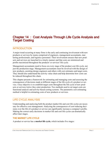
Final ANL/ESD/11-11December 20112.2Data Sources and Key Parameters Associated with Natural Gas RecoveryThe EPA develops the U.S. GHG emissions inventory annually. This effort accumulateslarge amounts of GHG data as EPA develops methodologies to estimate emissions for differentsectors, including the oil, coal, and NG sectors. The EPA methodologies and data are widelyused by others, including by us, for performing GHG analyses of specific energy systems. Asummary of key emission factors considered in the recovery of natural gas is provided inTable 1. Each stage and the assumptions behind its associated emissions are described inSections 2.2.4 and 2.2.5.TABLE 1Selected Activity Factors for the Recovery of Natural GasStageSample Emission Sources for Shale and Conventional GasUnless Otherwise NotedWell CompletionsDrill out methane (CH4) ventingFlow back CH4 venting (shale only)WorkoversCH4 ventingLiquid UnloadingCH4 venting (conventional only)Miscellaneous VentingField separation equipmentGathering compressorsNormal operationsCondensate collectionCompressor ventingUpsetsFlaringCarbon dioxide (CO2) emissionsIn its most recent inventory estimation, EPA made major methodological changes to howit analyzes the total CH4 emissions of the U.S. NG system (EPA 2011). While EPA’s CH4emission factors for the U.S. NG system are based primarily on a joint study by the gas industryand EPA (Harrison et al. 1996), the EPA updates activity factors, such as length of theU.S. pipeline network and number of producing gas wells, on an annual basis. EPA also makesminor adjustments to emission factors where appropriate and includes additional CH4 sourceswhen data become available. We note that in its 2011 inventory estimation, EPA made asignificant upward adjustment of CH4 emissions from the U.S. NG system, such that total CH4emissions more than doubled from levels used in the previous inventory. Table 2 presents thechanges to selected EPA emission factors.4

Final ANL/ESD/11-11December 2011TABLE 2Comparison of Changes to Selected EPA Emissions Factors (EPA 2010b)Emissions SourcePreviousEmissions FactorRevisedEmissions FactorWell venting for liquids1.02unloadingGas venting during well completionsConventional well0.02110.71Unconventional well0.02177Gas venting during well workoversConventional well0.05Unconventional well0.05Centrifugal compressor0wet seal degassingventing0.05177233UnitsCH4 metric tons/year-wellCH4 metric tons/yearcompletionCH4 metric tons/yearcompletionCH4 metric tons/year-workoverCH4 metric tons/year-workoverCH4 metric tons/yearcompressorNote: Conversion factor of 0.01926 metric tons 1 Mcf.The underlying reasons for these adjustments are explained in Sections 2.2.4 and 2.2.5.Burdens associated with NG recovery as part of the EPA GHG inventory and those burdensoutside of the GHG inventory are detailed in the following subsections.Table 3 summarizes the key parameters that are discussed in the following subsectionsand are included in the natural gas pathways.5

Final ANL/ESD/11-11December 2011TABLE 3 Key Parameters for Natural Gas Simulation in GREET (mean values with ranges inparentheses)ParameterWell LifetimeBulk Gas MethaneContentProduction over WellLifetime (estimatedultimate recovery)Well Completion andWorkovers (venting)CH4 Reductions forCompletion orWorkoversNumber of Workoversper well lifetimeLiquid Unloadings(venting)Liquid UnloadingEventsCH4 Reductions forLiquid UnloadingsWells RequiringUnloadingsWell Equipment(leakage and venting)CH4 Reductions forWell EquipmentWell Equipment (CO2from flaring)Well Equipment (CO2from venting)Processing (leakageand venting)Processing (CO2 fromventing)Transmission andStorage (leakage andventing)Distribution (leakageand ustry andArgonneAssumption%85 (69–95)80 (40–97)Hanle 2011NG million onv: EIA 2011b;Shale: ChesapeakeEnergy 2010Metric ton CH4per completion orworkover0.71177(13.5–385)EPA 2010b%041 (37–70)EPA 2011;EPA 2010a22EPA 2010b0.860EPA 2010b31 (11–51)0EPA 2010b%12 (8–15)0EPA 2011;EPA 2010a%41.30EPA 2010bGrams CH4 permillion Btu NG209(114–303)209(114–303)%28 (18–37)28 (18–37)Grams CO2 permillion Btu NGGrams CO2 permillion Btu NGCH4: % of NGproducedGrams CO2 permillion Btu NG454(369–538)454(369–538)GAO 2010;EPA 2011EPA 2011;EPA 2010aGAO 2010;EPA 20114141EPA 23)878(615–1140)CH4: % of NGproduced0.39(0.2–0.58)0.39(0.2–0.58)EPA 2011CH4: % of NGproduced0.28(0.09–0.47)0.28(0.09–0.47)EPA 2011Workovers perlifetimeMetric ton CH4per unloadingUnloadings peryearEPA 2011EPA 2011Distribution accounts for leakage and venting from terminals to refueling stations. It does not apply to majorindustrial users, such as electricity generators.6

Final ANL/ESD/11-11December 20112.2.1 Estimated Ultimate RecoveryGiven that the EPA GHG inventory emissions from NG well completions and liquidunloadings are estimated on a per-well basis, it was necessary to determine the estimatedultimate recovery (EUR) of gas from a well to amortize these periodic emissions over the totalamount of natural gas produced. For shale gas wells, a range was developed for EURs accordingto the per-well weighted average of four major plays: Marcellus, Barnett, Haynesville, andFayetteville. The high estimates were based upon industry average–targeted EURs(Mantell 2010b). The low estimates were based upon a review of emerging shale resourcesdeveloped by INTEK, Inc., for the EIA (INTEK 2011). The INTEK analysis captured thevariability in EUR within a play by evaluating the EUR for the best area, the average area, andthe below-average area in a play. INTEK further presented EURs for active portions andundeveloped portions of major plays, and generally, the active portions of the play had largerEURs than did the undeveloped areas. Comparing the EURs with the industry average–targetedEURs, the active EURs reported in INTEK were similar, with the exception of the Marcellusplay. While the active reported EURs reported by INTEK were lower for the Marcellus than theindustry average–targeted EUR, the industry average–targeted EUR was contained within therange of EURs presented for the best, average, and below-average EURs for the Marcellusdeveloped area. We averaged the high and low values to estimate our Base Case shale gas wellEUR of 3.5 billion cubic feet (Bcf), as shown in Table 4.TABLE 4 Lifetime Production Estimates According to Play (INTEK 2011; Mantell 2010b)Low EUR Estimates (Bcf)High EUR Estimates 6Haynesville3.56.5Per-Well Weighted Average1.65.3The estimates in Table 4 are for the bulk gas, which is a mixture containing methane inaddition to other gases such as ethane, propane, carbon dioxide, and nitrogen.For the conventional NG EUR, we assumed an average production rate over the lifetimeof the well according to EIA production data and EPA well compositional makeup, recognizingthat production rates typically decline over time, to estimate a Base Case EUR of 1.6 Bcf(EPA 2011, EIA 2011b). Our estimate of conventional EUR is comparable to a value from ananalysis of Texas wells prior to large-scale shale gas production (Swindell 2001). It should benoted when comparing the EURs that shale gas recovery typically uses horizontal drilling toaccess large rock volumes, whereas conventional gas recovery often uses multiple vertical wells,each accessing a smaller rock volume. To account for these differences and enable comparison,7

Final ANL/ESD/11-11December 2011the analysis evaluates impacts on a per-million-Btu (mmBtu) basis. In addition, in the case ofconventional gas, it may be that the highly productive wells have ceased production and modernwells return relatively less gas, as shown by the fall in the EUR for Texas over the years(Swindell 2001). As the large-scale recovery of NG from shale plays is a relatively new pursuit,the EUR may not reflect future conditions when the technologies that support large-scale shalegas recovery are more mature. For emissions associated with processing, transmission, storage,and distribution, we based our emissions calculations on total production of shale gas (SG) andNG as we did not need to differentiate by gas source (EIA 2011b).2.2.2 Well Design, Drilling, and ConstructionThe drilling phase of the NG life cycle requires the use of drill rigs, fuel, and materials,including the casing, cement, liners, mud constituents, and water. Water is used during the wellconstruction stage in drilling fluids, for cementing the casing in place, and for hydraulicallyfracturing the well in the case of shale gas. For the purposes of our analysis, the horizontal shalegas wells were based on designs for the 4H, 5H, and 6H Carol Baker wells and modifiedaccording to the depth of the shale play (Range Resources 2011a–c). For horizontal drilling, awell is drilled down to the depth of the play and turned approximately 90 degrees to run laterally(horizontally) through the play for 2,000 to 6,500 feet (ft). Vertical wells draw from a muchsmaller area within a play. The conventional NG scenario assumed a vertical well design, whichwas based upon a design from the Mississippi Smackover and adjusted to the national averagedepth of gas wells (Bourgoyne et al. 1991; EIA 2011b). Because of the long lateral reach ofhorizontal wells, they can access more of the play, which typically increases production on a perwell basis.The total volume of drilling muds, or fluids, used to lubricate and cool the drill bit,maintain downhole hydrostatic pressure, and convey drill cuttings from the bottom of the hole tothe surface depends upon the volume of the borehole and the physical and chemical properties ofthe formation. The ratio of barrels (bbl) of drilling mud to bbl of annular void used in thisassessment was 5:1 according to data obtained from the literature (EPA 1993). The materialinventory assumes use of water-based fluids for the Barnett and Haynesville plays. Analysis ofthe Marcellus and Fayetteville plays assumes use of air drilling through the upper portion of thewell to a depth of 392 ft and water drilling below that depth (GWPC and ALL 2009). For thewater-based drilling muds, a ratio of 1 bbl of water to 1 bbl of drilling mud was assumed. Thecomposition of the mud was adapted from Mansure (2010) to provide the required drilling fluidproperties. The dominant material — by several orders of magnitude — was bentonite; as aresult, the other materials were ignored for this study.8

Final ANL/ESD/11-11December 2011To determine fuel consumption, the following assumptions were made: The drill rig operates with a 2,000-horsepower (hp) engine,The engine consumes diesel fuel at a rate of 0.06 gallon (gal)/hp/hour (h), andThe drill rig runs at 45% of capacity.These assumptions are similar to those reported by Tester et al. (2006), EPA (2004a), andRadback Energy (2009). By assuming that the drill rig operates 24 hours per day and then usingan average number of days drilled from Overbey et al. (1992) and extrapolating to the variousplays according to depth, the total diesel fuel required for drilling can be determined. Althoughdiesel fuel requirements for on-site activities and transportation burdens for diesel and waterwere included in the inventory, the transportation burdens of materials (e.g. mud, cement, steel)were not included. The summary of materials, water, and fuel used to drill and construct thehorizontal wells is presented in Table 5.TABLE 5 Material Requirements for Drilling and Constructing a Typical Well by Play (units arein metric tons per well unless otherwise indicated)Shale GasWell DrillingBarnett163Steel267Portland CementGilsonite9(asphaltite)Diesel Fuel61,768(gallons)61.38Bentonite1.06Soda Ash0.04Gelex1.60Polypac0.81Xanthum GumWater (throughput269,693in gallons per well)aaConventional ter volumes do not account for water associated with hydraulic fracturing activities.2.2.3 Hydraulic Fracturing and Management of Flowback WaterBecause of the low permeabilities of shale formations, which limit the flow of NG withinthe formation, producers hydraulically fracture the formation to enable the flow of NG. Thisoutcome is accomplished by pumping fracture fluid at a predetermined rate and pressuresufficient to create fractures in the target formation. The fracture fluid for shale formations istypically water based and consists of proppants, sand, or similarly sized engineered particles thatmaintain fracture openings once they have been established and the pumping of fracture fluid has9

Final ANL/ESD/11-11December 2011ceased. Although we included the transportation and management burdens for water andflowback from hydraulic fracturing activities, we did not include the production andtransportation burdens of proppants and other chemicals, because the small amounts ofconsumption involved would affect the results only minimally.For this analysis, values for fracturing (or frac) fluid constituents were based uponfraccing data made available by Range Resources, which released frac fluid information forseveral of its Marcellus wells (Range Resources 2010a–c). Large volumes of water are requiredfor drilling and fraccing activities. Typical volumes depend on the characteristics of the shaleand are provided in Table 6.TABLE 6Typical Range of Water Requirements Per Well for FraccingActivities by Shale Play (GWPC & ALL 2009, Mantell 2010b)Shale PlayBarnettMarcellusFayettevilleHaynesvilleTypical Range of Frac Water Input per Well 02,900,000–4,200,0002,700,000–5,000,000The total water input varies according to geology and drilling practices, with air drillingcommonly practiced in the Marcellus and Fayetteville plays. While the constituents of a frac jobwill vary according to site conditions, the average concentrations of these constituents wereextrapolated to other shale plays according to typical water use for a relatively similar frac ineach play. The estimated components and amounts for frac jobs in the Marcellus are presented inTable 7.10

Final ANL/ESD/11-11December 2011TABLE 7 Estimated Fraccing Fluid Components According to AverageValues from Selected Marcellus Wells (Range Resources 2010a–c)Per WellWaterSandFriction Reducer (polyacrylamide, mineral oil)Antimicrobial AgentGlutaraldehyden-alkyl dimethyl benzyl ammonium yde AmineScale InhibitorSodium hydroxideEthylene glycolPerforation Cleanup37% HClMethanolPropargyl algalgalgalgalgalgalgalgalgalgalgalBecause of the relatively small amounts of chemicals per mmBtu, the life-cycle energyand emissions burdens of the proppants and components of fracturing fluids were not included.However, the energy and emissions burdens a

conventional natural gas liquid unloadings — that need to be addressed further. Our base case results show that shale gas life-cycle emissions are 6% lower than those of conventional natural gas. However, the range in values for shale and conventional gas overlap, so there is a statistical