Transcription
THE PHYSICS OF WAVESVersion date - February 15, 2015
THE PHYSICS OF WAVESHOWARD GEORGIHarvard UniversityOriginally published byPRENTICE HALLEnglewood Cliffs, New Jersey 07632
c 1993 by Prentice-Hall, Inc.⃝A Simon & Schuster CompanyEnglewood Cliffs, New Jersey 07632All rights reserved. No part of this book may bereproduced, in any form or by any means,without permission in writing from the publisher.Printed in the United States of America10 9 8 7 6 5 4 3Prentice-Hall International (UK) Limited, LondonPrentice-Hall of Australia Pty. Limited, SydneyPrentice-Hall Canada Inc., TorontoPrentice-Hall Hispanoamericana, S.A., MexicoPrentice-Hall of India Private Limited, New DelhiPrentice-Hall of Japan, Inc., TokyoSimon & Schuster Asia Pte. Ltd., SingaporeEditora Prentice-Hall do Brasil, Ltda., Rio de Janeiro
Contents1 Harmonic OscillationPreview . . . . . . . . . . . . . . . . . . . .1.1 The Harmonic Oscillator . . . . . . . .1.2 Small Oscillations and Linearity . . . .1.3 Time Translation Invariance . . . . . .1.3.1 Uniform Circular Motion . . . .1.4 Complex Numbers . . . . . . . . . . .1.4.1 Some Definitions . . . . . . . .1.4.2 Arithmetic . . . . . . . . . . .1.4.3 Complex Exponentials . . . . .1.4.4 Notation . . . . . . . . . . . .1.5 Exponential Solutions . . . . . . . . . .1.5.1 * Building Up The Exponential1.5.2 What is H? . . . . . . . . . . .1.6 LC Circuits . . . . . . . . . . . . . . .1.7 Units — Displacement and Energy . . .1.7.1 Constant Energy . . . . . . . .1.7.2 The Torsion Pendulum . . . . .1.8 A Simple Nonlinear Oscillator . . . . .Chapter Checklist . . . . . . . . . . . . . . .Problems . . . . . . . . . . . . . . . . . . .1125991212141518182223252829293032332 Forced Oscillation and ResonancePreview . . . . . . . . . . . . . . . . . . .2.1 Damped Oscillators . . . . . . . . . .2.1.1 Overdamped Oscillators . . .2.1.2 Underdamped Oscillators . . .2.1.3 Critically Damped Oscillators2.2 Forced Oscillations . . . . . . . . . .37373738394142v.
CONTENTSvi2.3Resonance . . . . . . . . . . . . . . .2.3.1 Work . . . . . . . . . . . . .2.3.2 Resonance Width and Lifetime2.3.3 Phase Lag . . . . . . . . . . .2.4 An Example . . . . . . . . . . . . . .2.4.1 Feeling It In Your Bones . . .Chapter Checklist . . . . . . . . . . . . . .Problems . . . . . . . . . . . . . . . . . .44454547484851513 Normal ModesPreview . . . . . . . . . . . . . . . . . . . . .3.1 More than One Degree of Freedom . . . .3.1.1 Two Coupled Oscillators . . . . .3.1.2 Linearity and Normal Modes . . .3.1.3 n Coupled Oscillators . . . . . .3.2 Matrices . . . . . . . . . . . . . . . . . .3.2.1 * Inverse and Determinant . . . .3.2.2 More Useful Facts about Matrices3.2.3 Eigenvalue Equations . . . . . . .3.2.4 The Matrix Equation of Motion .3.3 Normal Modes . . . . . . . . . . . . . .3.3.1 Normal Modes and Frequencies .3.3.2 Back to the 2 2 Example . . . .3.3.3 n 2 — the General Case . . . .3.3.4 The Initial Value Problem . . . .3.4 * Normal Coordinates and Initial Values .3.4.1 More on the Initial Value Problem3.4.2 * Matrices from Vectors . . . . .3.4.3 * ω 2 is Real . . . . . . . . . . . .3.5 * Forced Oscillations and Resonance . . .3.5.1 Example . . . . . . . . . . . . .Chapter Checklist . . . . . . . . . . . . . . . .Problems . . . . . . . . . . . . . . . . . . . .5353545457585962656667687072757677798081828386874 SymmetriesPreview . . . . . . . . . . . . . . . .4.1 Symmetries . . . . . . . . . . .4.1.1 Beats . . . . . . . . . .4.1.2 A Less Trivial ExampleChapter Checklist . . . . . . . . . . .9393939899104.
CONTENTSviiProblems . . . . . . . . . . . . . . . . . . . . . . . . . . . . . . . . . . . . . . . 1045 WavesPreview . . . . . . . . . . . . . . . . . . . . . . . . . . . . . . . . .5.1 Space Translation Invariance . . . . . . . . . . . . . . . . . . .5.1.1 The Infinite System . . . . . . . . . . . . . . . . . . . .5.1.2 Boundary Conditions . . . . . . . . . . . . . . . . . . .5.2 k and Dispersion Relations . . . . . . . . . . . . . . . . . . . .5.2.1 The Dispersion Relation . . . . . . . . . . . . . . . . .5.3 Waves . . . . . . . . . . . . . . . . . . . . . . . . . . . . . . .5.3.1 The Beaded String . . . . . . . . . . . . . . . . . . . .5.3.2 Fixed Ends . . . . . . . . . . . . . . . . . . . . . . . .5.4 Free Ends . . . . . . . . . . . . . . . . . . . . . . . . . . . . .5.4.1 Normal Modes for Free Ends . . . . . . . . . . . . . . .5.5 Forced Oscillations and Boundary Conditions . . . . . . . . . .5.5.1 Forced Oscillations with a Free End . . . . . . . . . . .5.5.2 Generalization . . . . . . . . . . . . . . . . . . . . . .5.6 Coupled LC Circuits . . . . . . . . . . . . . . . . . . . . . . .5.6.1 An Example of Coupled LC Circuits . . . . . . . . . .5.6.2 A Forced Oscillation Problem for Coupled LC CircuitsChapter Checklist . . . . . . . . . . . . . . . . . . . . . . . . . . . .Problems . . . . . . . . . . . . . . . . . . . . . . . . . . . . . . . 321331341356 Continuum Limit and Fourier SeriesPreview . . . . . . . . . . . . . . . . . .6.1 The Continuum Limit . . . . . . . .6.1.1 Philosophy and Speculation6.2 Fourier series . . . . . . . . . . . .6.2.1 The String with Fixed Ends6.2.2 Free Ends . . . . . . . . . .6.2.3 Examples of Fourier Series .6.2.4 Plucking a String . . . . . .Chapter Checklist . . . . . . . . . . . . .Problems . . . . . . . . . . . . . . . . .1391391391411411411421441481491497 Longitudinal Oscillations and SoundPreview . . . . . . . . . . . . . . . . . . . .7.1 Longitudinal Modes in a Massive Spring7.1.1 Fixed Ends . . . . . . . . . . .7.1.2 Free Ends . . . . . . . . . . . .153153153155156.
CONTENTSviii7.27.3A Mass on a Light Spring . . . . . . .The Speed of Sound . . . . . . . . . .7.3.1 The Helmholtz Approximation7.3.2 Corrections to Helmholtz . . .Chapter Checklist . . . . . . . . . . . . . .Problems . . . . . . . . . . . . . . . . . .8 Traveling WavesPreview . . . . . . . . . . . . . . . . . . . .8.1 Standing and Traveling Waves . . . . .8.1.1 What is It That is Moving? . . .8.1.2 Boundary Conditions . . . . . .8.2 Force, Power and Impedance . . . . . .8.2.1 * Complex Impedance . . . . .8.3 Light . . . . . . . . . . . . . . . . . . .8.3.1 Plane Waves . . . . . . . . . .8.3.2 Interferometers . . . . . . . . .8.3.3 Quantum Interference . . . . .8.4 Transmission Lines . . . . . . . . . . .8.4.1 Parallel Plate Transmission Line8.4.2 Waves in the Transmission Line8.5 Damping . . . . . . . . . . . . . . . .8.5.1 Free Oscillations . . . . . . . .8.5.2 Forced Oscillation . . . . . . .8.6 High and Low Frequency Cut-Offs . . .8.6.1 More on Coupled Pendulums .Chapter Checklist . . . . . . . . . . . . . . .Problems . . . . . . . . . . . . . . . . . . 1841851861881901911921931931971989 The Boundary at InfinityPreview . . . . . . . . . . . . . . . . . . . . . . .9.1 Reflection and Transmission . . . . . . . . .9.1.1 Forced Oscillation . . . . . . . . . .9.1.2 Infinite Systems . . . . . . . . . . . .9.1.3 Impedance Matching . . . . . . . . .9.1.4 Looking at Reflected Waves . . . . .9.1.5 Power and Reflection . . . . . . . . .9.1.6 Mass on a String . . . . . . . . . . .9.2 Index of Refraction . . . . . . . . . . . . . .9.2.1 Reflection from a Dielectric Boundary.201201202202202204206207209211212.
CONTENTS9.3* Transfer Matrices . . . . . . . . .9.3.1 Two Masses on a String . .9.3.2 k Changes . . . . . . . . .9.3.3 Reflection from a Thin Film9.3.4 Nonreflective Coating . . .Chapter Checklist . . . . . . . . . . . . .Problems . . . . . . . . . . . . . . . . .ix.21321321621821922022110 Signals and Fourier AnalysisPreview . . . . . . . . . . . . . . . . . . .10.1 Signals in Forced Oscillation . . . . .10.1.1 A Pulse on a String . . . . . .10.1.2 Fourier integrals . . . . . . .10.2 Dispersive Media and Group Velocity10.2.1 Group Velocity . . . . . . . .10.3 Bandwidth, Fidelity, and Uncertainty .10.3.1 A Solvable Example . . . . .10.3.2 Broad Generalities . . . . . .10.4 Scattering of Wave Packets . . . . . .10.4.1 Scattering from a Boundary .10.4.2 A Mass on a String . . . . . .10.5 Is c the Speed of Light? . . . . . . . .Chapter Checklist . . . . . . . . . . . . . .Problems . . . . . . . . . . . . . . . . . 1 Two and Three DimensionsPreview . . . . . . . . . . . . . . . . . . . . . . . . . . . . . .11.1 The ⃗k Vector . . . . . . . . . . . . . . . . . . . . . . . .11.1.1 The Difference between One and Two Dimensions11.1.2 Three Dimensions . . . . . . . . . . . . . . . . .11.1.3 Sound Waves . . . . . . . . . . . . . . . . . . . .11.2 Plane Boundaries . . . . . . . . . . . . . . . . . . . . . .11.2.1 Snell’s Law — the Translation Invariant Boundary11.2.2 Prisms . . . . . . . . . . . . . . . . . . . . . . . .11.2.3 Total Internal Reflection . . . . . . . . . . . . . .11.2.4 Tunneling . . . . . . . . . . . . . . . . . . . . . .11.3 Chladni Plates . . . . . . . . . . . . . . . . . . . . . . . .11.4 Waveguides . . . . . . . . . . . . . . . . . . . . . . . . .11.5 Water . . . . . . . . . . . . . . . . . . . . . . . . . . . .11.5.1 Mathematics of Water Waves . . . . . . . . . . . .253253254256258260261263267270272276282284285
CONTENTSx11.5.2 Depth . . . . . . . . .11.6 Lenses and Geometrical Optics11.7 Rainbows . . . . . . . . . . .11.8 Spherical Waves . . . . . . . .11.9 Chapter Checklist . . . . . . .Chapter Checklist . . . . . . . . . .Problems . . . . . . . . . . . . . .28629230731431631631712 PolarizationPreview . . . . . . . . . . . . . . . . . . . . . . . . . . . . .12.1 The String in Three Dimensions . . . . . . . . . . . . .12.1.1 Polarization . . . . . . . . . . . . . . . . . . . .12.2 Electromagnetic Waves . . . . . . . . . . . . . . . . . .12.2.1 General Electromagnetic Plane Waves . . . . . .12.2.2 Energy and Intensity . . . . . . . . . . . . . . .12.2.3 Circular Polarization and Spin . . . . . . . . . .12.3 Wave Plates and Polarizers . . . . . . . . . . . . . . . .12.3.1 Unpolarized Light . . . . . . . . . . . . . . . .12.3.2 Polarizers . . . . . . . . . . . . . . . . . . . . .12.3.3 Wave Plates . . . . . . . . . . . . . . . . . . . .12.3.4 Matrices . . . . . . . . . . . . . . . . . . . . . .12.3.5 Optical Activity . . . . . . . . . . . . . . . . . .12.3.6 Crossed Polarizers and Quantum Mechanics . . .12.4 Boundary between Dielectrics . . . . . . . . . . . . . .12.4.1 Polarization Perpendicular to the Scattering Plane12.4.2 Polarization in the Scattering Plane . . . . . . .12.5 Radiation . . . . . . . . . . . . . . . . . . . . . . . . .12.5.1 Fields of moving charges . . . . . . . . . . . . .12.5.2 The Antenna Pattern . . . . . . . . . . . . . . .12.5.3 * Checking Maxwell’s equations . . . . . . . . .Chapter Checklist . . . . . . . . . . . . . . . . . . . . . . . .Problems . . . . . . . . . . . . . . . . . . . . . . . . . . . 5235435535536036136336413 Interference and DiffractionPreview . . . . . . . . . . . .13.1 Interference . . . . . . .13.1.1 The Double Slit .13.1.2 Fourier Optics .13.2 Beams . . . . . . . . . .13.2.1 Making a Beam .369369370370372374374.
CONTENTS13.2.2 Caveats . . . . . . . . . . . . . .13.2.3 The Boundary at . . . . . . .13.2.4 The Boundary at z 0 . . . . . .13.3.1 Small z . . . . . . . . . . . . . .13.3.2 Large z . . . . . . . . . . . . . .13.3.3 * Stationary Phase . . . . . . . .13.3.4 Spot Size . . . . . . . . . . . . .13.3.5 Angles . . . . . . . . . . . . . .13.4 Examples . . . . . . . . . . . . . . . . .13.4.1 The Single Slit . . . . . . . . . .13.4.2 Near-field Diffraction . . . . . . .13.4.3 The Rectangle . . . . . . . . . .13.4.4 δ “Functions” . . . . . . . . . . .13.4.5 Some Properties of δ-Functions .13.4.6 One Dimension from Two . . . .13.4.7 Many Narrow Slits . . . . . . . .13.5 Convolution . . . . . . . . . . . . . . . .13.5.1 Repeated Patterns . . . . . . . . .13.6 Periodic f (x, y) . . . . . . . . . . . . . .13.6.1 Twisting the Grating . . . . . . .13.6.2 Resolving Power . . . . . . . . .13.6.3 Blazed Gratings . . . . . . . . . .13.7 * X-ray Diffraction . . . . . . . . . . . .13.8 Holography . . . . . . . . . . . . . . . .13.9 Fringes and Zone Plates . . . . . . . . . .13.9.1 The Holographic Image of a Point13.9.2 Zone Plates . . . . . . . . . . . .Chapter Checklist . . . . . . . . . . . . . . . .Problems . . . . . . . . . . . . . . . . . . . .14 Shocks and WakesPreview . . . . . . . . . . . . . . . . . . . . .14.1 * Boat Wakes . . . . . . . . . . . . . . .14.1.1 Wakes . . . . . . . . . . . . . . .14.1.2 Linear analysis of the Kelvin wake14.1.3 Shocks versus Wakes . . . . . . .14.2 Chapter Checklist . . . . . . . . . . . . .Chapter Checklist . . . . . . . . . . . . . . . .Problems . . . . . . . . . . . . . . . . . . . 3423425437438438438
xiiCONTENTSBibliography440A The Programs443B Solitons447C Goldstone Bosons451
PrefaceWaves are everywhere. Everything waves. There are familiar, everyday sorts of waves inwater, ropes and springs. There are less visible but equally pervasive sound waves and electromagnetic waves. Even more important, though only touched on in this book, is the wavephenomenon of quantum mechanics, built into the fabric of our space and time. How can itmake sense to use the same word — “wave” — for all these disparate phenomena? What isit that they all have in common?The superficial answer lies in the mathematics of wave phenomena. Periodic behaviorof any kind, one might argue, leads to similar mathematics. Perhaps this is the unifyingprinciple.In this book, I introduce you to a deeper, physical answer to the questions. The mathematics of waves is important, to be sure. Indeed, I devote much of the book to the mathematicalformalism in which wave phenomena can be described most insightfully. But I use the mathematics only as a tool to formulate the underlying physical principles that tie together manydifferent kinds of wave phenomena. There are three: linearity, translation invariance and local interactions. You will learn in detail what each of these means in the chapters to come.When all three are present, wave phenomena always occur. Furthermore, as you will see,these principles are a great practical help both in understanding particular wave phenomenaand in solving problems. I hope to convert you to a way of thinking about waves that willpermanently change the way you look at the world.The organization of the book is designed to illustrate how wave phenomena arise in anysystem of coupled linear oscillators with translation invariance and local interactions. Webegin with the single harmonic oscillator and work our way through standing wave normalmodes in more and more interesting systems. Traveling waves appear only after a thoroughexploration of one-dimensional standing waves. I hope to emphasize that the physics ofstanding waves is the same. Only the boundary conditions are different. When we finally getto traveling waves, well into the book, we will be able to get to interesting properties veryquickly.For similar reasons, the discussion of two- and three-dimensional waves occurs late inthe book, after you have been exposed to all the tools required to deal with one-dimensionalwaves. This allows us at least to set up the problems of interference and diffraction in axiii
PREFACExivsimple way, and to solve the problems in some simple cases.Waves move. Their motion is an integral part of their being. Illustrations on a printedpage cannot do justice to this motion. For that reason, this book comes with moving illustrations, in the form of computer animations of various wave phenomena. These supplementaryprograms are an important part of the book. Looking at them and interacting with them, youwill get a much more concrete understanding of wave phenomena than can be obtained froma book alone. I discuss the simple programs that produce the animations in more detail inAppendix A. Also in this appendix are instructions on the use of the supplementary programdisk.The subsections that are illustrated with computer animations are clearly labeled in the.text by . and the number of the program. I hope you will read these parts of the book whilesitting at your computer screens.The sections and problems marked with acan be skipped by instructors who wish tokeep the mathematical level as low as possible.Two other textbooks on the subject, Waves, by Crawford and Optics by Hecht, influencedme in writing this book. The strength of Crawford’s book is the home experiments. Theseexperiments are very useful additions to any course on wave phenomena. Hecht’s book is anencyclopedic treatment of optics. In my own book, I try to steer a middle course betweenthese two, with a better treatment of general wave phenomena than Hecht and a more appropriate mathematical level than Crawford. I believe that my text has many of the advantagesof both books, but students may wish to use them as supplementary texts.While the examples of waves phenomena that we discuss in this book will be chosen(mostly) from familiar waves, we also will be developing the mathematics of waves in sucha way that it can be directly applied to quantum mechanics. Thus, while learning aboutwaves in ropes and air and electromagnetic fields, you will be preparing to apply the sametechniques to the study of the quantum mechanical world.I am grateful to many people for their help in converting this material into a textbook.Adam Falk and David Griffiths made many detailed and invaluable suggestions for improvements in the presentation. Melissa Franklin, Geoff Georgi, Kevin Jones and Mark Heald, alsohad extremely useful suggestions. I am indebted to Nicholas Romanelli for copyediting andto Ray Henderson for orchestrating all of it. Finally, thanks go to the hundreds of studentswho took the waves course at Harvard in the last fifteen years. This book is as much theproduct of their hard work and enthusiasm, as my own.*Howard GeorgiCambridge, MA
Preface to the online editionAs I prepared to teach the sophomore waves course at Harvard again after a break of over 10years, I realized that I had accumulated a list of many things that I wanted to change in mywaves text. And while I was very grateful to Prentice-Hall for all the help they gave me inturning my notes into a textbook, I felt that it was time to liberate the book from its paperstraightjacket, and try to turn it into something more continuously evolving. Thus I askedPrentice-Hall to release the rights back to me, and they graciously agreed. My intention is toleave the textbook up on the web for students and teachers to use as they see fit, so long asthey give me credit and do not use it for commercial purposes. I hope that readers will sendsuggestions for improvements. I will not have much time to think about these and implementthem. But if I do incorporate something in the online version as the result of a suggestion, Iwill acknowledge the suggestion in a list of changes on my web page.I have eliminated the table of contents from the online version and substituted hyperrefhypertext instead. I hope that this will encourage people to use the text online and save trees.Howard GeorgiCambridge, MADecember, 2006xv
Chapter 1Harmonic OscillationOscillators are the basic building blocks of waves. We begin by discussing the harmonicoscillator. We will identify the general principles that make the harmonic oscillator so special and important. To make use of these principles, we must introduce the mathematicaldevice of complex numbers. But the advantage of introducing this mathematics is that wecan understand the solution to the harmonic oscillator problem in a new way. We show thatthe properties of linearity and time translation invariance lead to solutions that are complexexponential functions of time.PreviewIn this chapter, we discuss harmonic oscillation in systems with only one degree of freedom.1. We begin with a review of the simple harmonic oscillator, noting that the equation ofmotion of a free oscillator is linear and invariant under time translation;2. We discuss linearity in more detail, arguing that it is the generic situation for smalloscillations about a point of stable equilibrium;3. We discuss time translation invariance of the harmonic oscillator, and the connectionbetween harmonic oscillation and uniform circular motion;4. We introduce complex numbers, and discuss their arithmetic;5. Using complex numbers, we find solutions to the equation of motion for the harmonicoscillator that behave as simply as possible under time translations. We call thesesolutions “irreducible.” We show that they are actually complex exponentials.6. We discuss an LC circuit and draw an analogy between it and a system of a mass andsprings.1
CHAPTER 1. HARMONIC OSCILLATION27. We discuss units.8. We give one simple example of a nonlinear oscillator.1.1 The Harmonic OscillatorWhen you studied mechanics, you probably learned about the harmonic oscillator. We willbegin our study of wave phenomena by reviewing this simple but important physical system.Consider a block with mass, m, free to slide on a frictionless air-track, but attached to a light1Hooke’s law spring with its other end attached to a fixed wall. A cartoon representation ofthis physical system is shown in figure 1.1. -. . . . . . . . . . . . . . . . . . . . . . . . . . . . . .Figure 1.1: A mass on a spring.This system has only one relevant degree of freedom. In general, the number of degrees of freedom of a system is the number of coordinates that must be specified in orderto determine the configuration completely. In this case, because the spring is light, we canassume that it is uniformly stretched from the fixed wall to the block. Then the only importantcoordinate is the position of the block.In this situation, gravity plays no role in the motion of the block. The gravitational forceis canceled by a vertical force from the air track. The only relevant force that acts on theblock comes from the stretching or compression of the spring. When the spring is relaxed,there is no force on the block and the system is in equilibrium. Hooke’s law tells us thatthe force from the spring is given by a negative constant, K, times the displacement of theblock from its equilibrium position. Thus if the position of the block at some time is x andits equilibrium position is x0 , then the force on the block at that moment isF K(x x0 ) .(1.1)1“Light” here means that the mass of the spring is small enough to be ignored in the analysis of the motionof the block. We will explain more precisely what this means in chapter 7 when we discuss waves in a massivespring.
1.1. THE HARMONIC OSCILLATOR3The constant, K, is called the “spring constant.” It has units of force per unit distance, orM T 2 in terms of M (the unit of mass), L (the unit of length) and T (the unit of time). Wecan always choose to measure the position, x, of the block with our origin at the equilibriumposition. If we do this, then x0 0 in (1.1) and the force on the block takes the simpler formF Kx .(1.2)Harmonic oscillation results from the interplay between the Hooke’s law force and Newton’s law, F ma. Let x(t) be the displacement of the block as a function of time, t. ThenNewton’s law impliesd2m 2 x(t) K x(t) .(1.3)dtAn equation of this form, involving not only the function x(t), but also its derivatives is calleda “differential equation.” The differential equation, (1.3), is the “equation of motion” for thesystem of figure 1.1. Because the system has only one degree of freedom, there is only oneequation of motion. In general, there must be one equation of motion for each independentcoordinate required to specify the configuration of the system.The most general solution to the differential equation of motion, (1.3), is a sum of aconstant times cos ωt plus a constant times sin ωt,x(t) a cos ωt b sin ωt ,(1.4) whereω Km(1.5)is a constant with units of T 1 called the “angular frequency.” The angular frequency will bea very important quantity in our study of wave phenomena. We will almost always denote itby the lower case Greek letter, ω (omega).Because the equation involves a second time derivative but no higher derivatives, themost general solution involves two constants. This is just what we expect from the physics,because we can get a different solution for each value of the position and velocity of theblock at the starting time. Generally, we will think about determining the solution in termsof the position and velocity of the block when we first get the motion started, at a time thatwe conventionally take to be t 0. For this reason, the process of determining the solutionin terms of the position and velocity at a given time is called the “initial value problem.”The values of position and velocity at t 0 are called initial conditions. For example, wecan write the most general solution, (1.4), in terms of x(0) and x′ (0), the displacement andvelocity of the block at time t 0. Setting t 0 in (1.4) gives a x(0). Differentiating andthen setting t 0 gives b ω x′ (0). Thusx(t) x(0) cos ωt 1 ′x (0) sin ωt .ω(1.6)
CHAPTER 1. HARMONIC OSCILLATION4For example, suppose that the block has a mass of 1 kilogram and that th
The organization of the book is designed to illustrate how wave phenomena arise in any system of coupled linear oscillators with translation invariance and local interactions. We begin with the single harmonic oscillator and work our way through standing wave normal modes in more and more int