Transcription
Data Quality for Index Models andMigration to Quantitative ModelsErnest Lever Thursday, June 15, 2017 API, 1800 West Loop South, Suite 475, Houston, TexasPHMSA RISK MODEL WORK GROUP
Agenda and Presentation FlowPHMSA RISK MODEL WORK GROUP2
ComplexityPHMSA RISK MODEL WORK GROUP
Definitions: Complexity The number of words we need todescribe a situation Complexity is closely related toinformation content Need a lot of words to describeeverything in this picture We need to describe each item asthey are different from the others Descriptions are at a small scalePHMSA RISK MODEL WORK GROUP4
Definitions: Complexity – Less Complex Need a fewer words to describeeverything in this picture There is more commonality There are common patterns atlarge scale Two colors Two teams FocusPHMSA RISK MODEL WORK GROUP5
Definitions: Complexity – Simple Need even fewer words to describethis picture Ignore the internal details of theperson Ignore the organization of the snowmolecules Only need the mass of the skier,the angle of the slope and theamount of frictionPHMSA RISK MODEL WORK GROUP6
Definitions: Complexity vs. ScalePHMSA RISK MODEL WORK GROUP7
Highly Engineered Systems – Very ComplexPHMSA RISK MODEL WORK GROUP8
Statistics Probability PhysicsPHMSA RISK MODEL WORK GROUP9
Predicting the FuturePHMSA RISK MODEL WORK GROUP
Why is The Past a Poor Predictor of the Future? There are at least two reasons why the past is a poor predictor of the future:1. Different system states due to interactions take a long time to manifestthemselves2. Independence of stochastic events with known probability pa) The current event is not influenced by the past – the process has no memoryb) In reality we infer unknown p from evaluation of the past eventsi.This is an uncertain process that we will address in upcoming slidesii.We may succumb to faulty logic in thinking that the past events actually do give us theprobability of occurrence pPHMSA RISK MODEL WORK GROUP11
System of Systems View In systems of systems there are many possible outcome states (COMPLEXITY) We need to enumerate all of these states We need to count how many times each state occurs (PROBABILITY) It takes many interactions over a long timeframe to see all states A purely empirical approach based on reaction to what has already happenedwill be blind to the majority of outcome states It we use a purely empirical approach we will be surprised by new lowerprobability outcome states We will not understand how they came to bePHMSA RISK MODEL WORK GROUP12
Progression of System Fault Severity Due to Sub-SystemInteractions Working assumption thatmore simultaneous subsystem faults that interactleads to greaterconsequence Backed up by NTSB andother investigations ofindustrial disastersPHMSA RISK MODEL WORK GROUP0 subsystemfaultsPerfectOperations1st subsystemfaultSimple Fault2nd subsystemfaultSignificantFault3rd subsystemfaultMajor Fault4th subsystemfaultCatastrophicFault5th subsystemfaultCatastrophicFault13
Spatio-Temporal Simulation of Interactions Simulate a system with fivesub-systems Each has a 30 year expectedlifetime (50% likelihood ofsystem anomaly) Each has a different rate ofreaching 50% likelihood ofsystem anomaly in 30 years Use logistic distributions tomodel each sub-systemPHMSA RISK MODEL WORK GROUP14
Cumulative Interactions Over 30 Years 10,000 spatial locationswhere five sub-systemscan interact 1,000 simulations ofpossible combinations ofthe sub-system states ateach spatial location 10,000,000 totalinteractions evaluated Count the numberoccurrences of0, 1, 2 ,3,4 or 5 faults at alocationPHMSA RISK MODEL WORK GROUP15
One in a Million Threshold for Cumulative Interactions 1 system fault always exceeds1 10 6 likelihood ofoccurrence10,000,000 interactions were evaluated.The one in a million threshold is 10 partsin 10,000,000 – the maximum z axisbound in the current plot. 2 interacting faults – in year 3 3 interacting faults – in year13 4 interacting faults – in year19 5 interacting faults – in year25PHMSA RISK MODEL WORK GROUP16
Interactions in Each One Year Timeframe Count the number ofoccurrences of0, 1, 2 ,3,4 or 5 faults at alocation in each one yeartimeframePHMSA RISK MODEL WORK GROUP17
One in a Million Threshold for Interactions in a Specific Year 1 system fault alwaysexceeds 1 10 6likelihood of occurrence 2 interacting faults – inyear 5 3 interacting faults – inyear 17 4 interacting faults – inyear 23 5 interacting faults – inyear 27PHMSA RISK MODEL WORK GROUP10,000,000 interactions were evaluated.The one in a million threshold is 10 partsin 10,000,000 – the maximum z axisbound in the current plot.18
Tabular Depiction of the Information in thePrevious Four SlidesPHMSA RISK MODEL WORK GROUP19
Probability Distributions:Predicting the Next OutcomePHMSA RISK MODEL WORK GROUP
How to Develop Distributions for Risk Models We need to identify possible system states Each time we inspect the system it is either in aparticular state or not We count each outcome separately –is in state k, is notin state k This is a Bernoulli processA Bernoulli process is a finite or infinite sequence of independent random variables X1, X2, X3, .,such that For each i, the value of Xi is either 0 or 1; For all values of i, the probability that Xi 1 is the same number p.In other words, a Bernoulli process is a sequence of independent identically distributed Bernoullitrials.Independence of the trials implies that the process is memoryless. Given that the probability p isknown, past outcomes provide no information about future outcomes. (If p is unknown,however, the past informs about the future indirectly, through inferences about p.)https://en.wikipedia.org/wiki/Bernoulli processPHMSA RISK MODEL WORK GROUP21
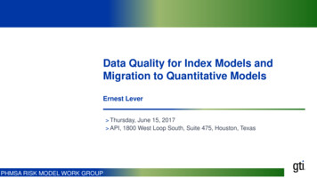
The Past Informs About the Future Indirectly, ThroughInferences About p Counting the number of times asystem is in state k gives anestimate of the probability p ofbeing in state k How certain are we about thisinference? Bayesian Inference using theBeta distribution quantifies theuncertainty in our inferencePHMSA RISK MODEL WORK GROUPIn Bayesian inference, the beta distribution is the conjugate prior probabilitydistribution for the Bernoulli, binomial, negative binomial and geometricdistributions. For example, the beta distribution can be used in Bayesian analysisto describe initial knowledge concerning probability of success such as theprobability that a space vehicle will successfully complete a specified mission. Thebeta distribution is a suitable model for the random behavior of percentages andproportions.https://en.wikipedia.org/wiki/Beta distributionP 4/6 2/3.(1-p) 1/322
Beta(4,2) and Beta(5,3) The Beta distribution has 0.667LCB0.2840.290UCB0.9470.901Beta(5,3) Beta(alpha, beta) Alpha – count of successes Beta – count of non-successes𝑚𝑒𝑎𝑛 𝛼𝛼 𝛽𝑚𝑜𝑑𝑒 PHMSA RISK MODEL WORK GROUP𝛼 1𝛼 𝛽 2Beta(4,2)23
How to Develop Beta Distributions from Data1. Start by defining our initial beliefabout the probability of success orfailurea) In the absence of solid knowledge usean ignorant prior: Beta(1,1)b) An ignorant prior defines the state wherewe have a 50% probability of success orfailure, but any proportion of success orfailure is equally likelyc) In other words we do not have a cluePHMSA RISK MODEL WORK GROUP24
Bayesian Updating for the Beta Distribution is Simpleand Painless2. Setup a simple spreadsheet3. Enter an ignorant prior in the first cellsCredible Bounds4. Use the Excel function BETA.INV(D 1,B4,C4)to calculate the credible bounds5. Calculate the mean directly from the 0.0250.5000.975TRUE /FALSEN/ACredible Bounds0.95 (1-C1)/2 1-D1Data PointAlphaBetaLCBMeanUCBTRUE / FALSE0121 IF(G5 CHAR(32),B4 G5,CHAR(32)) IF(G6 CHAR(32),B5 G6,CHAR(32))1 IF(G5 CHAR(32),C4 (1-G5),CHAR(32)) IF(G6 CHAR(32),C5 (1-G6),CHAR(32)) BETA.INV(D 1,B4,C4) IF(G5 CHAR(32),BETA.INV(D 1,B5,C5),CHAR(32)) IF(G6 CHAR(32),BETA.INV(D 1,B6,C6),CHAR(32)) IF(G4 CHAR(32),B4/(B4 C4),CHAR(32)) IF(G5 CHAR(32),B5/(B5 C5),CHAR(32)) IF(G6 CHAR(32),B6/(B6 C6),CHAR(32)) BETA.INV(E 1,B4,C4) IF(G5 CHAR(32),BETA.INV(E 1,B5,C5),CHAR(32)) IF(G6 CHAR(32),BETA.INV(E 1,B6,C6),CHAR(32))N/A CHAR(32) CHAR(32)PHMSA RISK MODEL WORK GROUP25
Bayesian Updating for the Beta Distribution is Simpleand Painless6. Increment the Alpha column by 1 for asuccessful outcome7. Increment the Beta column by one foran unsuccessful outcomeCredible Bounds95%0.0250.975Data 5000.6670.5000.9750.9870.906TRUE /FALSEN/ATRUEFALSECredible Bounds0.95Data Point012Alpha1 IF(G5 CHAR(32),B4 G5,CHAR(32)) IF(G6 CHAR(32),B5 G6,CHAR(32)) (1-C1)/2Beta1 IF(G5 CHAR(32),C4 (1-G5),CHAR(32)) IF(G6 CHAR(32),C5 (1-G6),CHAR(32))PHMSA RISK MODEL WORK GROUP 1-D1LCB BETA.INV(D 1,B4,C4) IF(G5 CHAR(32),BETA.INV(D 1,B5,C5),CHAR(32)) IF(G6 CHAR(32),BETA.INV(D 1,B6,C6),CHAR(32))Mean IF(G4 CHAR(32),B4/(B4 C4),CHAR(32)) IF(G5 CHAR(32),B5/(B5 C5),CHAR(32)) IF(G6 CHAR(32),B6/(B6 C6),CHAR(32))UCBTRUE / FALSE BETA.INV(E 1,B4,C4) IF(G5 CHAR(32),BETA.INV(E 1,B5,C5),CHAR(32)) IF(G6 CHAR(32),BETA.INV(E 1,B6,C6),CHAR(32))26N/ATRUEFALSE
Bayesian Updating for an inspection ProcessCredible 2232425262728293095%0.0250.975Inspection 50.5570.5400.5240.5080.4940.5140.333TRUE 0.333TRUE10.333PHMSA RISK MODEL WORK GROUP27
PHMSA RISK MODEL WORK GROUP28
Example of Beta Distributions and Bayesian UpdatingUsed to Evaluate Risk Under Uncertainty 22 out of 365 fusions failed inservice Random sampling plandeveloped to assess qualityof non-failed fusions Hypergeometric distributionused to predict findingsbased on prior data –equivalent to an exact Fishertest for significancePHMSA RISK MODEL WORK GROUP29
Credible Bounds for Sub-Populations and EntirePopulation Credible bounds for each subpopulation heavily impacted bynumber of samples All results are statistically significantat the 0.05 level per thehypergeometric prior probabilities Can combine sub-populations as theinstallations were performed by asingle contractor, using a singleprocess in the same time frame.PHMSA RISK MODEL WORK GROUPSize1614121086Entire Population(Not additive withresults bilityof Failure2.5% LowerCredibleBound97.5% 5.5%99.5%97.6%93.02%81.4%99.2%30
Incorporating Data Quality MetricsPHMSA RISK MODEL WORK GROUP31
Simple Scoring of Data Quality Attributes At the March meeting of theRisk Model Work Group wediscussed methods forassigning data quality scores We can subjectively choose aline of demarcation for theWeights Score : 12.5 Good 12.5 BadPHMSA RISK MODEL WORK GROUP32
How to Implement the Data Quality Score For an poorly understood system the data qualityscore is arrived at through an audit process How do we extrapolate the audit results to thesystem as a whole?PHMSA RISK MODEL WORK GROUP33
Two Sub-Systems: 5,000 Data Aggregations Each Sub-system 1: Use the following stationary distribution : 90 Audits 60 Bad 30 Good Sub-system 2: 6 Audits 2 Bad 4 Good This distribution estimates the number ofsystem components k out of a total of Nthat are in a good state given Dnegative (Down) and U positive (Up)influences (Bad and Good audit resultsrespectively) The distribution behaves very similarly tothe Beta distributionPHMSA RISK MODEL WORK GROUPHarmon, D., et al., Predicting economic marketcrises using measures of collective panic. 2011.34
Probability Distribution for The Audit Results Example The two probability densityfunctions obtained for thetwo audit cases presentedcan be used to simulatelocations with good dataquality based on the auditresultsPHMSA RISK MODEL WORK GROUP35
PHMSA RISK MODEL WORK GROUP36
What to do with the Data Quality Distribution Results This is a risk tolerance discussionthat has to tie back in to theRisk Governance/Risk Management/Risk Assessmentframework of the organization.PHMSA RISK MODEL WORK GROUP37
How to Address the Risk Tolerance Problem Address the organization, processes, andthe physical system Select program/data quality measuresand periodically evaluate them Quantify the causal relationship of rootcauses of each threat Incorporate the historical data, subjectmatter expert opinion, and belief aboutcollected data Consider the interactive nature of threatsPHMSA RISK MODEL WORK GROUP38
Risk Assessment of a Pipeline SystemPHMSA RISK MODEL WORK GROUP39
Simplified Process WorkflowPHMSA RISK MODEL WORK GROUP40
Data Entity RelationshipsPHMSA RISK MODEL WORK GROUP41
Process is Readily AutomatedPHMSA RISK MODEL WORK GROUP42
Node by Node Data Quality Consideration Conceptually, greater data quality measure value means higher confidence about the data, which is equivalent to smaller 𝜎 value inlikelihood function Assume the data quality of each threat is determined by a Beta distribution 𝐵𝑒𝑡𝑎 𝛼𝑖 , 𝛽𝑖𝛼𝑖𝐷𝑄𝑖 𝑚𝑒𝑎𝑛 𝛼𝑖 𝛽𝑖 𝛼𝑖 and 𝛽𝑖 will be updated based on the value of data quality measures such as authenticity, compliance, reliability, transparency, andpedigree For continuous nodes, introduce a measurement error 𝜎(1 "DQ" ) For ranked nodes, adjust probability histogram to increase/decrease uncertaintyPHMSA RISK MODEL WORK GROUP43
Data Quality Effect – Can be Extended to ConsequenceMeasures for Benefit/Cost Analysis of Improved Data QualityPHMSA RISK MODEL WORK GROUP44
Direct Tie in to Six Sigma Approaches To investigate the effect of likelihood function, it is assumedthat the pressure of a pipeline system follow a normaldistribution 𝜃 𝑁 𝜇0 , 𝜎0 2 Assume the value from the measurement system 𝑥 ′ 𝑥′ 𝜃 𝜀 where the measurement error term 𝜀 𝑁 0, 𝜎 Therefore, the posterior distribution of the pressure given themeasurement 𝑥 ′ is given as𝜎 2 𝜇0 𝜎0 2 𝑥 ′ 2(𝜃 )(𝜃 𝜇0 )2(𝑥 ′ 𝜃)2𝜎0 2 𝜎 2𝑝 𝜃 𝑥 exp( )exp( ) exp( )𝜎 2𝜎 22 𝜎0 22 𝜎22 2 0 2𝜎0 𝜎 The uncertainty of the posterior distribution depends on𝜎2 𝜎0 2.𝜎0 2 𝜎 2 It is trivial to show that values of 𝜎 produce higher uncertaintyin the posterior distribution 𝜃PHMSA RISK MODEL WORK GROUP45
Subject Matter ExpertisePHMSA RISK MODEL WORK GROUP46
Biases and Heuristics (Kahneman and Tversky 1982) Ambiguity effect—The avoidance of options for which missinginformation makes the probability seem unknown. Attentional bias—Neglect of relevant data when making judgments of a correlation orassociation. Availability heuristic—Estimating what is more likely bywhat is more available in memory, which is biased toward vivid, unusual,or emotionally charged examples. Base rate neglect—Failing to takeaccount of the prior probability. This was at the heart of the commonfallacious reasoning in the Harvard medical study described in Chapter 1.It is the most common reason for people to feel that the results ofBayesian inference are nonintuitive. Bandwagon effect—Believingthings because many other people do (or believe) the same. Related togroupthink and herd behavior. Confirmation bias—Searching for orinterpreting information in a way that confirms one’s preconceptions. Déformation professionnelle—Ignoring any broader point of view andseeing the situation through the lens of one’s own professional norms. Expectation bias—The tendency for people to believe, certify, andpublish data that agrees with their expectations. This is subtly different toconfirmation bias, because it affects the way people behave before theyconduct a study. Framing—By using a too narrow approach ordescription of the situation or issue. Also framing effect, which is drawingdifferent conclusions based on how data are presented. Need forclosure—The need to reach a verdict in important matters; to have ananswer and to escape the feeling of doubt and uncertainty. The personalcontext (time or social pressure) might increase this bias. Outcomebias—Judging a decision by its eventual outcome instead of based onthe quality of the decision at the time it was made. Overconfidenceeffect—Excessive confidence in one’s own answers to questions. Forexample, for certain types of question, answers that people rate as 99%certain turn out to be wrong 40% of the time. Status quo bias—Thetendency for people to like things to stay relatively the same.Fenton, Norman. Risk Assessment and Decision Analysis with Bayesian Networks (Page 262). Taylor and Francis CRC ebook account. Kindle EditionPHMSA RISK MODEL WORK GROUP47
Comparing Expert Models It is possible to construct hybrid Bayesiannetworks that compare the performance ofcompeting expert models given different dataFenton, Norman. Risk Assessment and Decision Analysis with Bayesian Networks (Page 320 - 324).Taylor and Francis CRC ebook account. Kindle EditionPHMSA RISK MODEL WORK GROUP48
OptimizationPHMSA RISK MODEL WORK GROUP49
How to Optimize Risk Reduction Activities This is a vast topic with many well defined solution approaches that wecannot even begin to address adequately in a single session Monte Carlo simulation can be used to good effect in evaluating a largenumber of alternative approaches It is important to evaluate many diverse approaches and identify whichapproach is best in particular situations (SITUATIONAL AWARENESS) Constant Bayesian updating of the underlying probability distributionsand re-running simulations is helpful Causal networks will help define the optimization problem better Approaches that reduce system variance will have great effect Prompt mitigation and repair of identified system anomalies will helpreduce the likelihood of higher order system interactions that can beproblematicPHMSA RISK MODEL WORK GROUP50
Applying the Causal Framework to ArmageddonFenton, Norman. Risk Assessment and Decision Analysis with Bayesian Networks (Page 46). Taylor and Francis CRC ebook account. KindleEdition. Risk measurement is more meaningful in thecontext; the BN tells a story that makes sense.This is in stark contrast with the simple “riskequals probability times impact” approachwhere not one of the concepts has a clearunambiguous interpretation. Uncertainty isquantified and at any stage we can simply readoff the current probability values associated withany event. It provides a visual and formalmechanism for recording and testing subjectiveprobabilities. This is especially important for arisky event that you do not have much or anyrelevant data about (in the Armageddonexample this was, after all, mankind’s firstmission to land on a meteorite).PHMSA RISK MODEL WORK GROUP51
KUUUB Factors and Other operational RisksFenton, Norman. Risk Assessment and Decision Analysis with Bayesian Networks (Chapter 11). Taylor and Francis CRC ebook account.Kindle Edition. Known Unknowns Unknown Unknowns BiasPHMSA RISK MODEL WORK GROUP52
Discussion and QuestionsPHMSA RISK MODEL WORK GROUP53
Additional Slides On IntegratingData Quality into Risk AsessmentPHMSA RISK MODEL WORK GROUP54
Stochastic Risk Analysis ofGas Pipeline with BayesianStatisticsPHMSA RISK MODEL WORK GROUP55
Deterministic Risk Analysis Most common quantitative risk assessment method Estimates single-point value for discrete scenarios such as worst case, bestcase, and most likely outcomes Considers only a few outcomes, ignoring all other possibilities Disregards interdependence between inputs Ignores uncertainty in input variablesPHMSA RISK MODEL WORK GROUP56
Stochastic Risk Analysis with Bayesian Statistics Advanced quantitative risk assessment method Estimates probability distribution of the risk By using probability distributions, variables can have different probabilities of differentoutcomes Uncertainties in variables are described by probability distributions Probabilistic results show not only what could happen, but how likely each outcome is Allows scenario analysis and sensitivity analysis Possible to model interdependent relationships between input variablesPHMSA RISK MODEL WORK GROUP57
Bayesian Statistics Quantitative tool to rationally update subjective prior beliefs in light of new evidence.Posterior Prior Likelihood𝑃 𝐷 𝑃 𝐷 𝑃( )/𝑃(𝐷) is the parameterP( ) is the priorP( D) is the posteriorP(D ) is the likelihoodP(D) is the evidencePHMSA RISK MODEL WORK GROUP58
Illustrative Pipeline Network for Example in FollowingSlides Synthetic gas pipeline networkof 120 components (e.g.,joints, piping, etc) divided into: 3 regions 4 segments per region 10 components per segment Risk analysis can be performedat component level, segmentlevel, or region levelPHMSA RISK MODEL WORK GROUP59
Component Failure Threat Types from ASME B31.8SStandard Time-Dependent Threats Internal Corrosion External Corrosion Stress Corrosion Cracking Time-Independent Threats Incorrect Operations Procedure Weather and Outside Force Third Party Damage Resident Threats Manufacturing Defects Construction or Fabrication Defects Equipment FailurePHMSA RISK MODEL WORK GROUP60
Probability of Component Failure Probability of Failure over time 𝑡𝑝𝑛𝑚 𝑗 𝑡 𝑖 1 𝑘 1 𝑤𝑗, 𝑘1𝑓 𝑡𝑖 , 𝑥𝑗, 𝑦𝑘 𝑑𝑦 𝑑𝑥 𝑑𝑡 x, y, and t represents threat type, input variable, and time instance respectively. [t1, tp] is the time interval for which likelihood of failure is calculated n is the total number of threat type ( 9 for gas pipeline per AMSE B31.8S) m is the total number of input variables responsible for a given threat type where wj,k is the weight applied for each input variable from threat model f(t, x, y) is calculated from the Beta distribution of component failure attribute asshown in the next few slides.PHMSA RISK MODEL WORK GROUP61
Probability of Component Failure1. Determine prior belief P( ) on parameters [0,1] where is always eithersuccess (1) or failure (0) Beta distribution quantifies the prior beliefs for binomial outcome. The probability density function of the beta distribution is𝑃(𝜃 𝛼, 𝛽) 𝜃α 1(1 𝜃)β 1/𝐵(𝛼, 𝛽)where 𝐵(𝛼, 𝛽) acts a normalizing constant so that the area under PDFsums to one. Initially, ignorant prior of 𝐵(𝛼 1, 𝛽 1) is used in the very first run.PHMSA RISK MODEL WORK GROUP62
Probability of Component Failure2. Determine likelihood function. Bernoulli distribution is well-suited for the Boolean-valued outcomeusually labelled as ‘success’ (1) and ‘failure’ (0), in which it takes thevalue 1 with probability p and the value 0 with probability 1-p. The probability mass function of the distribution is𝑓 𝑘, 𝑝 𝑝𝑘 1 𝑝where 𝑘 {1,0}.PHMSA RISK MODEL WORK GROUP1-k63
Probability of Component Failure3. Determine posterior probability function of [0,1]. Posterior Prior Likelihood𝑃 𝑃 𝐷 𝑃 𝐷 𝑤ℎ𝑒𝑟𝑒, P(D) 𝑃 𝐷, 𝑑 𝑃 𝐷 Bernoulli likelihood and Beta prior are conjugate pairs – as a result, the posterior is a Betadistribution. The conjugate priors simplifies the calculation of posterior distribution. The computation of posterior distribution is a complex process (example, integration forP(D)) and therefore a numerical approximation method instead such as Markov ChainMonte Carlo (MCMC) is needed. 𝑃𝑜𝑠𝑡𝑒𝑟𝑖𝑜𝑟 𝐵𝑒𝑡𝑎 𝑑𝑖𝑠𝑡𝑟𝑖𝑏𝑢𝑡𝑖𝑜𝑛 𝑀𝐶𝑀𝐶 𝐵𝑒𝑡𝑎 𝑝𝑟𝑖𝑜𝑟, 𝐵𝑒𝑟𝑛𝑜𝑢𝑙𝑙𝑖 𝑙𝑖𝑘𝑒𝑙𝑖ℎ𝑜𝑜𝑑PHMSA RISK MODEL WORK GROUP64
Probability of Component Failure using Markov ChainMonte CarloMetropolis-Hastings algorithm1. Begin the algorithm at the current position in parameter space (θcurrent)2. Propose a "jump" to a new position in parameter space (θnew)3. Accept or reject the jump probabilistically using the prior information andavailable data4. If the jump is accepted, move to the new position and return to step 15. If the jump is rejected, stay at current position and return to step 16. After a set number of jumps have occurred, return all ofthe accepted positionsPHMSA RISK MODEL WORK GROUP65
Probability Distribution of Component FailurePHMSA RISK MODEL WORK GROUP66
Consequence of FailuresFive Categories of Consequences Very Low Low Medium High Very HighPHMSA RISK MODEL WORK GROUP67
Stochastic Risk Analysis𝑅𝑖𝑠𝑘 Probability 𝑜𝑓 𝐹𝑎𝑖𝑙𝑢𝑟𝑒 𝐶𝑜𝑛𝑠𝑒𝑞𝑢𝑒𝑛𝑐𝑒 𝑜𝑓 𝐹𝑎𝑖𝑙𝑢𝑟𝑒PHMSA RISK MODEL WORK GROUP68
Implication of Data Quality in Risk Analysis Integrity Authenticity Compliance Transparency Reliability PedigreePHMSA RISK MODEL WORK GROUP Beta Distribution 𝐵 𝛼, 𝛽 Start with 𝛼 1, 𝛽 1 𝛼 𝛼 1 𝑖𝑓 Authenticity 𝑇𝑅𝑈𝐸 1 𝑖𝑓 Compliance 𝑇𝑅𝑈𝐸 1 𝑖𝑓 Transparency 𝑇𝑅𝑈𝐸 1 𝑖𝑓 Reliability 𝑇𝑅𝑈𝐸 1 (𝑖𝑓 Pedigree 𝑇𝑅𝑈𝐸 ) 𝛽1111 𝛽 1 𝑖𝑓 Authenticity 𝐹𝐴𝐿𝑆𝐸 𝑖𝑓 Compliance 𝐹𝐴𝐿𝑆𝐸 𝑖𝑓 Transparency 𝐹𝐴𝐿𝑆𝐸 𝑖𝑓 Reliability 𝐹𝐴𝐿𝑆𝐸 𝑖𝑓 Pedigree 𝐹𝐴𝐿𝑆𝐸69
This is a Bernoulli process A Bernoulli process is a finite or infinite sequence of independent random variables X 1, X 2, X 3, ., such that For each i, the value of X i is either 0 or 1; For all values of i, the probability that X i 1 is the same number p. In other words, a Bernoulli process is a sequence of independent identically .