Transcription
This is a preprint of an article that has appeared in The Journal of Computational Finance 17 (1), 43-70, ue-1-2013A MONTE CARLO PRICING ALGORITHM FOR AUTOCALLABLESTHAT ALLOWS FOR STABLE DIFFERENTIATIONTHOMAS ALM†, BASTIAN HARRACH‡, DAPHNE HARRACH† AND MARCO KELLER†Abstract. We consider the pricing of a special kind of options, the so-called autocallables, whichmay terminate prior to maturity due to a barrier condition on one or several underlyings. StandardMonte Carlo (MC) algorithms work well for pricing these options but they do not behave stable withrespect to numerical differentiation. Hence, to calculate sensitivities, one would typically resort toregularized differentiation schemes or derive an algorithm for directly calculating the derivative.In this work we present an alternative solution and show how to adapt a MC algorithm in sucha way that its results can be stably differentiated by simple finite differences. Our main tool is theone-step survival idea of Glasserman and Staum which we combine with a technique known as GHKImportance Sampling for treating multiple underlyings.Besides the stability with respect to differentiation our new algorithm also possesses a significantlyreduced variance and does not require evaluations of multivariate cumulative normal distributions.Key words. Monte Carlo, Autocallables, Express Certificate, sensitivities, stable differentiation,one-step survival, GHK importance sampling, variance reduction1. Introduction. The application of Monte Carlo (MC) simulation to optionpricing started with a paper by Boyle [4] who was the first to use MC to price European call options on dividend paying stocks as an extension to the analytical solutionfor options on non-dividend paying stocks published in the seminal Black-Scholes paper four years before [2]. Boyle already stressed the point that it is advisable to gobeyond the standard MC approach by applying techniques to effectively reduce thevariance, reasoning however ”that it is not possible to formulate general rules regarding the selection and implementation of the most effective technique“ [4]. A variety oftechniques already known from areas other than option pricing have been successfullyadopted to improve the MC pricing for various types of uni- and multivariate options.Some new techniques have been developed to price specific types of exotic options,making use of distinct features of their respective payoffs. For an overview about thevarious approaches we refer to the monograph by Glasserman [9].Within this paper, we will consider MC pricing schemes for so-called autocallableoptions. Autocallables have been traded intensely in particular in the market forstructured retail derivatives (certificates). As an example, autocallables, which areknown under the trade name of Express Certificates in the German market for retailcertificates made up for more than 30% of this market in 2008, see, e.g., Wegnerand Alm [1] for an overview. Most of the certificates of this type issued had oneunderlying (Single Express Certificates), some had two underlyings (Duo ExpressCertificates). Autocallables with one, resp., multiple underlyings are also called uni-,resp., multivariate.The name autocallable refers to the fact that, just as with a normal callable bond,the autocallable can be terminated prior to its maturity. The difference, however, isthat the autocallable is called automatically as soon as a certain barrier condition isfulfilled on one of some predefined observation dates, whereas a callable bond has tobe called by its issuer. More precisely, the idea of this type of financial instrumentis as follows (cf. figure 1.1): At specific points in time (the observation dates), it is† BHF-BANK, Frankfurt, Germany (thomas.alm@bhf-bank.com, marco.keller@bhf-bank.com anddaphne.von-harrach@bhf-bank.com)‡ Birth name: Bastian Gebauer, Department of Mathematics, Technische Universität München,Germany (harrach@ma.tum.de)1
This is a preprint of an article that has appeared in The Journal of Computational Finance 17 (1), 43-70, ue-1-20132T. Alm, B. Harrach, D. Harrach and M. Keller1st observation date: Underlying BarrierYesEarly Payoff 1No2nd observation date: Underlying BarrierYesEarly Payoff 2No.Nom-th observation date: Underlying BarrierYesPayoff mNoRedemption payment depending on final underlying priceFig. 1.1. Payoff profile of an autocallablechecked whether the underlying (resp., a function of several underlyings) reaches acertain barrier. If this is the case, the buyer of the autocallable gets a pre-definedconstant cash-flow (payoff) and the certificate terminates. Otherwise the instrumentcontinues to exist until the next observation date, and so forth. For those cases, wherethe autocallable survives until maturity, a payoff depending on the underlying(s)is generated at the maturity date. Autocallables can be considered as an exotictype of barrier options, cf., e.g., Zhang [17], the so-called window-barrier knock-outoptions with rebate, and with the number of windows corresponding to the number ofobservation dates, and each window having zero length. They are, however, typicallytreated as an option class of its own (see, e.g., Bouzoubaa and Osseiran [5]).We consider the pricing of autocallables under the standard assumption that theoption price is described by the discounted expected payoff using (correlated) geometric Brownian motion as the stochastic process for the underlyings, see, e.g. Hull[13]. For specific types of autocallables, analytical (closed-form) solutions have beenderived in Reder [15]. However, these solutions require the evaluation of multivariatecumulative normal distributions, with the dimension depending on the product of thenumber of underlyings and the number of observation dates. Higher-variate cumulative normal distributions require numerical methods (see, e.g., Genz and Bretz [7]) andare typically evaluated by Monte Carlo simulations. Since, furthermore, autocallablesare an option class which involves a variety of possible payoffs [5], this suggests touse Monte Carlo simulation as a generic way of pricing autocallables. However, itis worth mentioning that closed-form solutions, even if they exist for certain specialcases only, may serve as a useful input to improve Monte Carlo simulations, e.g., byusing control-variate methods.In this work, we derive an efficient Monte Carlo algorithm for pricing autocallables, and for calculating their sensitivities. In doing so, our goals are twofold.First, we aim at obtaining reliable prices with as few MC paths as possible. Second,we want to stably determine the option’s sensitivities such as Delta (derivative w.r.t.the price of the underlying) and Vega (derivative w.r.t. the option’s implied volatility)from the numerically calculated prices.Note that the second goal is particularly ambitious. Differentiation is generallyunstable, as even the smallest numerical errors in the price may have arbitrarily large
This is a preprint of an article that has appeared in The Journal of Computational Finance 17 (1), 43-70, ue-1-2013A Monte Carlo pricing algorithm for autocallables that allows stable differentiation3effects on the derivatives. In the mathematical literature this property is knownas ill-posedness, cf., e.g., Engl, Hanke and Neubauer [6], and, in general, requiressophisticated regularization strategies, cf., e.g., Hanke and Scherzer [12]. Our aim inthis work is, however, to design a MC pricing strategy that allows stable differentiationby simple finite differences.For the univariate express certificate, both our goals can be achieved using theideas of one-step survival established by Glasserman and Staum [10]. The idea isto restrict the Monte Carlo simulation to the survival zone (i.e., the area below thebarrier) and to treat the thus neglected contributions from the barrier analytically.In other words, instead of sampling from the full normal distribution, a truncatednormal distribution excluding values above the barrier is used. This approach yieldsa substantial variance reduction [10]. We will explain and numerically demonstratethat this approach also allows for stable differentiation. The main reason for thisbehaviour is that the discontinuity generated by any Monte Carlo path crossing thebarrier is avoided by construction.The main new part of this paper is to extend Glasserman and Staum’s onestep survival strategy to the multivariate case. The challenge of this extension ishow to sample from a truncated multivariate normal distribution without destroying the stability with respect to differentiation. In particular, as we explain in section 2.2, acception-rejection strategies fail in this task. Our tools to solve this challengestem from a technique known as GHK Importance Sampling Simulator (named afterGeweke, Hajivassiliou and Keane, see [8, 11, 14], and the concise description in Shum[16]). To the knowledge of the authors, this is the first time that the ideas of GHKare being adapted to the pricing of options via Monte Carlo simulations.Ultimately, we derive a Monte Carlo algorithm for multivariate autocallables thatallows stable differentiation by simple finite differences. We also numerically demonstrate that combining finite differences with our new algorithm is more efficient thandirectly calculating the option’s sensitivity with a likelihood ratio method. Moreover,our numerical experiments also show that, compared to standard MC algorithms, thenew algorithm possesses a substantially reduced variance. Since no evaluations ofmultivariate cumulative normal distributions are required, this variance reduction isachieved at the cost of only a moderately increased computation time, which indicatesthat our new algorithm is also an efficient way for pricing autocallables.The outline of this work is as follows. In section 2 we derive our new Monte Carlopricing algorithm for the univariate and the multivariate case, and discuss its stabilitywith respect to differentiation. Then, we numerically demonstrate our algorithms’stability and study its variance reduction properties in section 3. Section 4 containssome concluding remarks.2. Monte Carlo pricing of uni- and multivariate autocallable options.In this section, we derive our Monte Carlo pricing algorithm for autocallable options.Based on a combination of Glasserman and Staums’ one-step survival techniques [10]and the GHK Importance Sampling [8], we will obtain a substantial variance reductioneffect as well as the possibility to stably differentiate the numerically calculated pricesby simple finite differences.2.1. The univariate case. We start with the univariate case where the autocallable option depends on only one underlying. This subsection is more of anintroductory nature as the univariate case can be treated with a straight-forwardapplication of the one-step survival techniques in [10] to our specific type of option.We will, however, also use this subsection to elaborate on the estimator’s stability
This is a preprint of an article that has appeared in The Journal of Computational Finance 17 (1), 43-70, ue-1-20134T. Alm, B. Harrach, D. Harrach and M. Kellerproperties with respect to differentiation which will be a crucial point in the latergeneralization to the multivariate case.Let St describe the evolution of the underlying spot price and let (S1 , . . . , Sm ) bea vector containing its evaluations at some fixed, chronologically sorted, observationdates (t1 , . . . , tm ). We will only consider the Black-Scholes model, i.e., St is assumedto follow a geometric Brownian motion,dSt µdt σdWt ,Stwhere µ : r b, r denotes the risk-free interest rate, b is the dividend yield, σ 0 isthe volatility, and Wt is a standard Brownian motion. The extension of the followingresults to the case of non-constant, but deterministic, parameters is obvious and it alsoseems possible to extend them to stochastic parameters, cf. our concluding remarksin section 4.It is well known that this yields (for j 0, . . . , m 1) pσ2Sj 1 Sj expµ (tj 1 tj ) σ tj 1 tj Zj ,(2.1)2with independent standard normally distributed Zj . t0 and S0 s0 are the currenttime (w.l.o.g. t0 t1 ) and underlying price.The discounted payoff of a univariate autocallable option is given by (see againfigure 1.1)Q(S1 , . . . , Sm ) e r(tj t0 ) Qj e r(tm t0 ) q(Sm /Sref )(2.2)ififSi /Sref B Sj /SrefSj /Sref B i j, j 1, . . . , m,where Qj denotes the constant payoff that is paid if the performance Sj /Sref of theunderlying at time tj is, for the first time, greater than the barrier value B on anobservation date. The performance is measured relative to some reference value Srefwhich is, e.g., the spot price at the issue date of the autocallable. If the performanceSj /Sref stays below the barrier for all observation dates, then the holder of the optionreceives a redemption payoff q depending on the final performance Sm /Sref (see subsection 2.3 for the necessary smoothness conditions of q). Note that all of the followingholds (with minor modifications) if the barrier level depends on the observation date.The value P Vt0 of such an autocallable option, at the current time t0 , is given byits expected discounted payoffP Vt0 E [Q(S1 , . . . , Sm )] .The standard Monte Carlo estimator for P Vt0 is calculated by sampling a sequence of possible realizations (s1,n , . . . , sm,n ), n 1, . . . , N , of the random variables(S1 , . . . , Sm ) and approximating P Vt0 by the average payoffN1 XQ (s1,n , . . . , sm,n ) .N n 1(2.3)The sampling process is easily implemented by starting with the current underlyingprice s0 , and then using (2.1) to subsequently generate s1 up to sm . Obviously,
This is a preprint of an article that has appeared in The Journal of Computational Finance 17 (1), 43-70, ue-1-2013A Monte Carlo pricing algorithm for autocallables that allows stable differentiation5in doing so, it is not necessary to calculate sj 1 if already sj /Sref B. Thus,calculating each sample tuple (s1 , . . . , sm ) using (2.1) requires m or less samples zjfrom the standard normally distributed variable Zj . These samples can be generatedby setting zj Φ 1 (uj ), where uj is drawn from a uniform distribution over theinterval (0, 1), and Φ is the cumulative standard normal distribution.The one-step survival technique of Glasserman and Staum [10] applied to theunivariate autocallable improves the above standard Monte Carlo scheme by samplingonly paths which stay below the barrier B for all observation dates tj , i.e., paths whichdo not lead to an early payoff. For our case, this can be achieved by changing the laststep in the above description to!2ln(BSref /sj ) (µ σ2 )(tj 1 tj ) 1zj Φ (pj uj ) with pj : Φ, (2.4) σ tj 1 tjwhich corresponds to sampling the argument pj uj from a uniform distribution on therestricted interval (0, pj ).Note that pj P (Sj 1 /Sref B Sj sj ) also describes the probability thatthe underlying will stay below the barrier in the next step. As a consequence, thesampling of the Zj is done from a truncated univariate standard normal distributionfor which2ln(BSref /sj ) (µ σ2 )(tj 1 tj )Zj . σ tj 1 tj(2.5)Of course, this modification will bias the result unless we correct for the missingbarrier hits, which should have happened with a probability of 1 pj . To make upfor this fact, an accordingly weighted (j 1)-th premature payoff must be added tothe total payoff for this sample tuple, and all further payoffs for this sample must beweighted by pj . Hence, we replace (2.3) by the estimatorN1 X[PVt0 : Q̃ (s1,n , . . . , sm,n ) ,N n 1(2.6)which is subsequently denoted as the one-step survival MC estimator. The tuple(s1,n , . . . , sm,n ) is sampled according to the one-step survival strategy explained above,Q̃(s1 , . . . , sm )hh: (1 p0 ) e r(t1 t0 ) Q1 p0 (1 p1 ) e r(t2 t0 ) Q2 p1 (1 p2 )e r(t3 t0 ) Q3hiii . . . pm 2 (1 pm 1 ) e r(tm t0 ) Qm pm 1 e r(tm t0 ) q(sm /Sref ) . . . Lm e r(tm t0 ) q(sm /Sref ) m 1Xj 0Lj (1 pj ) e r(tj 1 t0 ) Qj 1(2.7)Qj 1and Lj : i 0 pi .We summarize a possible implementation in Algorithm 1.Mathematically, we can interpret the one-step survival strategy as an integralsplitting technique. We have thatZP Vt0 (s0 ) e r(t1 t0 )ϕ(z)P Vt1 (s1 (z)) dz,(2.8)R
This is a preprint of an article that has appeared in The Journal of Computational Finance 17 (1), 43-70, ue-1-20136T. Alm, B. Harrach, D. Harrach and M. KellerAlgorithm 1 One-step survival MC estimator for a univariate autocallable option.Initialize random seedfor n 1, . . . , N doPn : 0, L : 1for j 0, . . . , m 1 do . p : Φ ln(BSref /sj ) (µ σ 2 /2)(tj 1 tj )(σ tj 1 tj )Pn : Pn (1 p)Le r(tj 1 t0 ) Qj 1L : pLSample uj U (0, 1) sj 1 : sj exp µ σ 2 /2 (tj 1 tj ) σ tj 1 tj Φ 1 (puj )end forPn : Pn Le r(tm t0 ) q(sm /Sref )end forPN[return PVt0 : N1n 1 Pnwhere ϕ is the standard normal distribution, σ2(t1 t0 ) σ t1 t0 z ,s1 (z) : s0 expµ 2P Vt1 (s1 ) Q1 for s1 B, and, for s1 B, P Vt1 (s1 ) is given by an analog to (2.8).Splitting the integration domain accordingly yieldsZP Vt0 (s0 ) (1 p0 )e r(t1 t0 ) Q1 e r(t1 t0 )ϕ(z)P Vt1 (s1 (z)) dzs1 (z) BRwith p0 : s1 (z) B ϕ(z) dz as in (2.4). Since ϕ is no longer a probability density onthe restricted integration domain, we normalize the remaining integral and writeZϕ(z) r(t1 t0 ) r(t1 t0 )P Vt0 (s0 ) (1 p0 )eQ 1 p0 e1s (z) B P Vt1 (s1 (z)) dzR p0 1with the new properly normalized probability density ϕ(z)p0 1s1 (z) B corresponding toa sampling step with survival condition as explained above. This change to a newprobability density can also be interpreted as a special case of importance sampling,with p0 being the corresponding likelihood ratio (importance sampling weight). Byiteratively splitting the integral expression for P Vt1 , and the following observationtimes until maturity, in an analogous manner, and then applying the Monte Carlotechnique to the remaining conditional densities, we obtain the estimator (2.6).Glasserman and Staum prove in [10] that this estimator is unbiased and demonstrate that it possesses a significantly reduced variance compared to the standardestimator (at the price of only slightly increased computational effort).Let us now turn to a point that has not been examined in [10]. It is well knownthat the Black-Scholes model leads to a backward parabolic evolution, which smoothesout the discontinuities arising from the autocallable structure. Consequently, theoption price P Vt0 depends smoothly on the current underlying price s0 .To investigate the smoothness properties of the estimators in (2.3) and (2.6), letus consider the case of a single sample N 1 (and a fixed random seed). Varyings0 for the standard MC estimator (2.3) may lead to discontinuities at those points
This is a preprint of an article that has appeared in The Journal of Computational Finance 17 (1), 43-70, ue-1-2013A Monte Carlo pricing algorithm for autocallables that allows stable differentiation7s0 , where one of the later values, s1 to sm , agrees with the barrier level, since anarbitrarily small change in s0 may then cause or prevent the premature payoff. Theone-step survival estimator (2.6) does not have these discontinuities. All expressionsin (2.6) depend smoothly on s0 and u1 , . . . , um . In subsection 2.3 we will show thatthis smoothness property indeed yields stability with respect to finite differences.Of course, for a high number of Monte Carlo samples N , also the discontinuities ofthe standard MC estimator will be smoothed out and it will more and more resemblea smooth function of s0 . However, the process of differentiation amplifies even thesmallest discontinuities. In fact, we demonstrate in Section 3 that calculating thederivative with respect to the price of the underlying (the option’s Delta) by standardfinite differences leads to completely unfeasible results for the standard MC estimator,while giving stable results for the one-step survival estimator.Let us finish this subsection with some more remarks. First of all, similar arguments as above apply for the other parameters of our autocallable option andconsequently to the calculation of other option price sensitivities such as vega (sensitivity w.r.t. the implied volatility). Also, it should be noted that the discontinuitybehaviour already occurs in the simple case of determining the sensitivity Delta of aEuropean binary (also called digital) option. Binary options mature with some fixedpayoff if the underlying value is above the strike and pay nothing otherwise. Alsothere, combining finite differences with a standard Monte Carlo pricing routine leadsto unfeasibly oscillating results due to the discontinuity of the payoff function. Theone-step survival estimator, on the other hand, forces every Monte Carlo path to return zero, and adds the probability weighted payoff, which is already the exact price.Hence, independently of N , it always returns the exact price and thus allows stabledifferentiation.Finally, let us comment on alternative ways to obtaining sensitivities of autocallables. First of all, one can differentiate the analytical pricing formulas mentionedin the introduction. This involves computationally expensive evaluations of multivariate cumulative normal distributions, and is also not a very flexible approach, as it isrestricted to specific payoffs. On the other hand, it is possible to directly simulate thesensitivities of options also for discontinuous payoffs. The most prominent way to dothis is arguably the Likelihood Ratio Method (LRM), cf., e.g., Glasserman [9], whichrelies on the fact, that a standard Monte Carlo estimator for the price can be turnedinto an estimator for a sensitivity, by weighting the payoffs of each Monte Carlo pathwith a special weight. For the sensitivity delta, this weight, z1 (s0 σ t1 t0 ) 1 , isparticularly simple and does not depend on the option’s payoff structure at all, whichmakes the LRM a very flexible and generic method.However, our numerical results in section 3 show that the combination of finitedifferences with the one-step survival estimator yields clearly superior results compared to the LRM. Furthermore, from a practical point of view, the finite differencemethod has the advantage, that sensitivity calculations can be played back to the simulation of the option price. For this reason, it is frequently the method-of-choice indedicated risk systems used for front- or middle-office activities within financial institutions. Adapting the Monte Carlo pricing routines to allow for stable differentiationeases the integration of new option types in such systems.2.2. The multivariate case. We will now consider an autocallable option thatdepends on multiple underlyings. To keep things simple, we restrict ourselves to twounderlyings and assume that the premature payoffs depend only on the maximum orthe minimum of the underlying prices. Actually, to the knowledge of the authors,
This is a preprint of an article that has appeared in The Journal of Computational Finance 17 (1), 43-70, ue-1-20138T. Alm, B. Harrach, D. Harrach and M. Kelleralmost every multivariate autocallable in the German market (the Duo Express Certificates mentioned in the introduction) has its premature payoff depending on theminimum of two underlyings. We nevertheless treat the maximum case first to explainthe ideas of our new approach before turning to the more relevant, but also slightlymore complicated, minimum case. Let us also stress that the technique herein canalso be applied to a higher number of underlyings, more complicated premature payoff conditions, or non-constant parameters in the stochastic model, cf. our concludingremarks in section 4.(1)(2)Let (St , St ) describe the evolution of two underlying spot prices in a Black(1)(2)Scholes model, i.e., (St , St ) solves(1)dSt(1)St(1) µ1 dt σ1 dWt(2)dStand(2)St(2) µ2 dt σ2 dWt ,R(1)(2)with µ1 , µ2 , σ1 , σ2 0, and a two-dimensional Brownian motion (Wt , Wt )with zero drift and covariance matrix 1 ρ.(2.9)ρ 1(1)(1)Similar to the univariate case in subsection 2.1, we denote by (S1 , . . . , Sm ) andthe vectors containing the underlying prices at some fixed chronologically sorted observation dates (t1 , . . . , tm ). They satisfy (for j 0, . . . , m 1) pσ12(1)(1)(1)µ1 Sj 1 Sj exp,(2.10)(tj 1 tj ) σ1 tj 1 tj Zj2 pσ2(2)(2)(2)Sj 1 Sj expµ2 2 (tj 1 tj ) σ2 tj 1 tj Zj,(2.11)2(2)(2)(S1 , . . . , Sm )(1)(2)where (Zj , Zj ) are normally distributed with zero drift, and covariance matrix(1)(1)(2)(2.9). t0 , S0 s0 , and S0underlying prices.(2) s0are the current time (w.l.o.g. t0 t1 ), and2.2.1. Early payoff depending on the maximum of the underlyings. Wefirst consider a multivariate autocallable option with the following (discounted) payoff(1)(2)Q(S1 , S1 , . . .) e r(tj t0 ) Qj (1)(1)(2)(2) r(tm t0 )eq(Sm /Sref , Sm /Sref )(1)(1)(2)(2)(2.12)ififMi B MjMj B i j, j 1, . . . , m,where Mj : max{Sj /Sref , Sj /Sref }, and Qj is the constant payoff that is paid ifat time tj the performance of one of the underlyings is for the first time greater thanthe barrier level B on an observation date. The case where the barrier depends onthe minimum of the underlyings poses some subtle additional difficulties and will betreated further below. The redemption payoff q is assumed to be some function ofthe final underlying prices (again we refer to subsection 2.3 for necessary smoothnessconditions on q).There is an obvious generalization of the Glasserman-Staum survival techniquesexplained for the one-dimensional case in section 2.1. Starting with the current prices
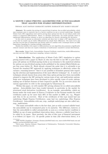
This is a preprint of an article that has appeared in The Journal of Computational Finance 17 (1), 43-70, ue-1-20139A Monte Carlo pricing algorithm for autocallables that allows stable differentiation(1)(2)(1)(2)(1)(2)(s0 , s0 ) we could subsequently generate samples (sj , sj ) of (Sj , Sj ) by using(1)(2)(2.10), (2.11), and the additional survival condition that, both, Sj 1 B and Sj 1 B. This boils down to sampling from a truncated multivariate normal distributionwith (k) (k)σ2ln BSref /sj µk 2k (tj 1 tj )(k)(k)pZj Cj : , k 1, 2,σk (tj 1 tj )and weighting payoffs according to the probability( (1))!(2) Sj 1 Sj 1(1)(2)(1) (2)(1)(2), BS,S s,s ΦC,C,P maxρjjjjjj(1)(2)Sref Srefwhere Φρ (·, ·) is the bivariate cumulative normal distribution with correlation ρ.However, there are two problems with this obvious generalization. The first one isthat it is not clear how to sample from a truncated multivariate normal distributionin a way that smoothly depends on all parameters, which is necessary to gain thedesired stability with respect to differentiation. In particular, acception-rejectionstrategies as proposed in [10] do not have this property. The second problem is thatthis approach requires the evaluation of a bivariate cumulative normal distributionfor every observation time and every MC sample, which is computationally expensive.This argument holds even more for the case of autocallables with more than two assets.Both problems can be solved by applying the ideas of GHK Importance Sampling[8], which enable us to sample one dimension after the other. To explain this approach, we proceed in reverse order of section 2.1. We start with an integral splittingargument, and, afterwards, interpret it as a one-step survival technique. We havethatZ (1) (2)(1)(2)P Vt0 (s0 , s0 ) e r(t1 t0 )ϕρ (z (1) , z (2) )P Vt1 s1 (z (1) ), s1 (z (2) ) d(z (1) , z (2) ),Rwhere(k)(k)s1 (z (k) ) s0 exp 2(2.13)µk σk22 (t1 t0 ) σk t1 t0 z (k) ,k 1, 2,(1)(2)ϕρ is the bivariate normal density with correlation ρ, P Vt1 Q1 for M (s1 , s1 ) B,and, otherwise, P Vt1 is given by an analog to (2.13).We apply the standard transformation to uncorrelated normal distributions,pz (1) y (1) and z (2) ρy (1) 1 ρ2 y (2) .This yields(1) (2)P Vt0 (s0 , s0 ) eZ r(t1 t0 )Rϕ(y(1))ZR (1) (2)ϕ(y (2) )P Vt1 s1 , s1dy (2) dy (1) ,(2.14)(k)(k)where now (with a slight abuse of notation) s1 s1(1)to(2)(1)(1) y (1) , y (2) , k 1, 2.(2)(2)The survival condition M (s1 , s1 ) max{s1 /Sref , s1 /Sref } B is equivalent(1)z (1) C1and(2)z (2) C1 ,
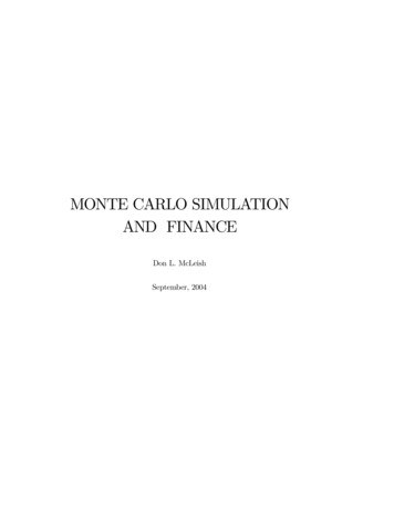
This is a preprint of an article that has appeared in The Journal of Computational Finance 17 (1), 43-70, ue-1-201310T. Alm, B. Harrach, D. Harrach and M. Keller2200 2 202 2 202Fig. 2.1. Survival zone before (left picture) and after (right picture) transformation to uncorrelated variables.and thus equivalent to(1)y (1) C1(2)andy (2) C1 ρy (1)p,1 ρ2see figure 2.1 for a sketch of these survival zones.We accordingly split the one-dimensional integrals in (2.14) and obtain by an easycalculation Z C1(1) (1) ϕ(y )(1) (2)(1) (2) r(t1 t0 )1 ppQ1P Vt0 (s0 , s0 ) e00(1) p0 (2) Z C1 ρy(1) (2)ϕ(y )1 ρ
type of barrier options, cf., e.g., Zhang [17], the so-called window-barrier knock-out options with rebate, and with the number of windows corresponding to the number of observation dates, and each window having zero length. They are, however, typically treated as an option class of its own (see, e.g., Bouzoubaa and Osseiran [5]).