WIXLIB

actions that run across multiple machines. The SAS Viya platform enables you to program with both CASactions and procedures, providing you with maximum flexibility to build an optimal ensemble.SAS Visual Data Mining and Machine Learning integrates CAS actions and CAS-powered proceduresand surfaces in-memory machine-learning techniques such as gradient boosting, factorization machines,neural networks, and much more through its interactive visual interface, SAS Studio tasks, procedures,and a Python client. This product bundle is an industry-leading platform for analyzing complex data,building predictive models, and conducting advanced statistical operations (Wexler, Haller, and Myneni2017).For more information about SAS Viya and SAS Visual Data Mining and Machine Learning, see thesection “Recommended Reading.” For specific code examples from this paper, refer to the Githubrepository referenced in that section.BUILDING A STRONG LIBRARY OF DIVERSE MODELSYou can generate a diverse set of models by using many different machine learning algorithms at varioushyperparameter settings. Forest and gradient bosting methods are themselves based on the idea ofcombining diverse decision tree models. The forest method generates diverse models by training decisiontrees on a number of bootstrap samples of the training set, whereas the gradient boosting methodgenerates a diverse set of models by fitting models to sequentially adjusted residuals, a form of stochasticgradient descent. In a broad sense, even multiple regression models can be considered to be anensemble of single regression models, with weights determined by least squares. Whereas the traditionalwisdom in the literature is to combine so-called “weak” learners, the modern approach is to create anensemble of a well-chosen collection of strong yet diverse models.In addition to using many different modeling algorithms, the diversity in a model library can be furtherenhanced by randomly subsetting the rows (observations) and/or columns (features) in the training set.Subsetting rows can be done with replacement (bootstrap) or without replacement (for example, k-foldcross validation). The word “bagging” is often used loosely to describe such subsetting; it can also beused to describe subsetting of columns. Columns can be subsetted randomly or in a more principledfashion that is based on some computed measure of importance. The variety of choices for subsettingcolumns opens the door to the large and difficult problem of feature selection.Each new big data set tends to bring its own challenges and intricacies, and no single fixed machinelearning algorithm is known to dominate. Furthermore, each of the main classes of algorithms has a set ofhyperparameters that must be specified, leading to an effectively infinite set of possible models you canfit. In order to navigate through this model space and achieve near optimal performance for a machinelearning task, a basic brute-force strategy is to first build a reasonably large collection of model fits acrossa well-designed grid of settings and then compare, reduce, and combine them in some intelligent fashion.A modern distributed computing framework such as SAS Viya makes this strategy quite feasible.AVOIDING LEAKAGE WHILE STACKINGA naïve ensembling approach is to directly take the predictions of the test data from a set of models thatare fit on the full training set and use them as inputs to a second-level model, say a simple regressionmodel. This approach is almost guaranteed to overfit the data because the target responses have beenused twice, a form of data leakage. The resulting model almost always generalizes poorly for a new dataset that has previously unseen targets. The following subsections describe the most common techniquesfor combatting leakage and selecting ensembles that will perform well on future data.SINGLE HOLDOUT VALIDATION SETThe classic way to avoid overfitting is to set aside a fraction of the training data and treat its target labelsas unseen until final evaluation of a model fitting process. This approach has been the main one availablein SAS Enterprise Miner from its inception, and it remains a simple and reliable way to assess modelaccuracy. It can be the most efficient way to compare models. It also is the way most data science3

competitions are structured for data sets that have a large number of rows.For stacked ensembling, this approach also provides a good way to assess ensembles that are made onthe dedicated training data. However, it provides no direct help in constructing those ensembles, nor doesit provide any measure of variability in the model performance metric because you obtain only a singlenumber. The latter concern can be addressed by scoring a set of bootstrap or other well-chosen randomsamples of the single holdout set.K-FOLD CROSS VALIDATION AND OUT-OF-FOLD PREDICTIONSThe main idea of cross validation is to repeat the single holdout concept across different folds of thedata—that is, to sequentially train a model on one part of the data and then observe the behavior of thistrained model on the other held-out part, for which you know the ground truth. Doing so enables you tosimulate performance on previously unseen targets and aims to decrease the bias of the learners withrespect to the training data.Assuming that each observation has equal weight, it makes sense to hold out each with equal frequency.The original jackknife (leave-one-out cross validation) method in regression holds out one observation ata time, but this method tends to be computationally infeasible for more complex algorithms and large datasets. A better approach is to hold out a significant fraction of the data (typically 10 or 20%) and divide thetraining data into k folds, where k is 5 or 10. The following simple steps are used to obtain five-fold crossvalidated predictions:1. Divide the training data into five disjoint folds of as nearly equal size as possible, and possibly alsostratify by target frequencies or means.2. Hold out each fold one at a time.3. Train the model on the remaining data.4. Assess the trained model by using the holdout set.Fitting and scoring for all k versions of the training and holdout sets provides holdout (crossvalidated) predictions for each of the samples in your original training data. These are known as out-offold (OOF) predictions. The sum of squared errors between the OOF predictions and true target valuesyields the cross validation error of a model, and is typically a good measure of generalizability.Furthermore, the OOF predictions are usually safely used as inputs for second-level stacked ensembling.You might be able to further increase the robustness of your OOF predictions by repeating the entirek-fold exercise, recomputing OOFs with different random folds, and averaging the results. However, youmust be careful to avoid possible subtle leakage if too many repetitions are done. Determining the bestnumber of repetitions is not trivial. You can determine the best number by doing nested k-fold crossvalidation, in which you perform two-levels of k-fold cross validation (one within the other) and assessperformance at the outer level. In this nested framework, the idea is to evaluate a small grid of repetitionnumbers, determine which one performs best, and then use this number for subsequent regular k-foldevaluations. You can also use this approach to help choose k if you suspect that the common values of 5or 10 are suboptimal for your data.Cross validation can be used both for tuning hyperparameters and for evaluating model performance.When you use the same data both for tuning and for estimating the generalization error with k-fold crossvalidation, you might have information leakage and the resulting model might overfit the data. To dealwith this overfitting problem, you can use nested k-fold cross validation—you use the inner loop forparameter tuning, and you use the outer loop to estimate the generalization error (Cawley and Talbot2010).BAGGING AND OUT-OF-BAG PREDICTIONSA technique similar in spirit to k-fold cross-validation is classical bagging, in which numerous bootstrapsamples (with replacement) are constructed and the out-of-bag (OOB) predictions are used to assessmodel performance. One potential downside to this approach is the uneven number of times each4

observation is held out and the potential for some missing values. However, this downside is usuallyinconsequential if you perform an appropriate number of bootstrap repetitions (for example, 100). Thistype of operation is very suitable for parallel processing, where with the right framework generating 100bootstrap samples will not take much more clock time than 10 seconds.AN APPROACH TO BUILDING A STRONG, DIVERSE MODEL LIBRARYEXAMPLE: ADULT SALARY DATA SETThis section describes how to build a strong and diverse model library by using the Adult data set fromthe UCI Machine Learning Repository (Lichman 2013). This data set has 32,561 training samplesand16,281 test samples; it includes 13 input variables, which are a mix of nominal and interval variablesthat include education, race, marital status, capital gain, and capital loss. The target is a binary variablethat takes a value of 1 if a person makes less than 50,000 a year and value of 0 otherwise. The trainingand test set are available in a GitHub repository, for which a link is provided in the section“Recommended Reading.”Treating Nominal VariablesThe data set includes six nominal variables that have various levels. The cardinality of the categoricalvariables is reduced by collapsing the rare categories and making sure that each distinct level has at least2% of the samples. For example, the cardinality of the work class variable is reduced from 8 to 7, and thecardinality of the occupation variable is reduced from 14 to 12.The nominal variable education is dropped from the analysis, because the corresponding interval variable(education num) already exists. All the remaining nominal variables are converted to numerical variablesby using likelihood encoding as described in the next section.Likelihood Encoding and Feature EngineeringLikelihood encoding involves judiciously using the target variable to create numeric versions ofcategorical features. The most common way of doing this is to replace each level of the categoricalvariable with the mean of the target over all observations that have that level. Doing this carries a dangerof information leakage that might result in significant overfitting. The best way to combat the danger ofleakage is to perform the encoding separately for each distinct version of the training data during crossvalidation. For example, while doing five-fold cross validation, you compute the likelihood-encodedcategorical variable anew for each of the five training sets and use these values in the correspondingholdout sets. A drawback of this approach is the extra calculations and bookkeeping that are required.If the cardinality of a categorical variable is small relative to the number of observations and if the binarytarget is not rare, it can be acceptable to do the likelihood encoding once up front and run the risk of asmall amount of leakage. For the sake of illustration and convenience, that approach is taken here withthe Adult data set, because the maximum cardinality of the nominal variables is 12.Likelihood encoding has direct ties to classical statistical methods such as one-way ANOVA, and it canbe viewed as stacking the simple predictions from such models. More sophisticated versions involveshrinking the encoded means toward an overall mean, which can be particularly effective when the classsizes are imbalanced. This approach is well-known to improve mean square prediction error and ispopularly known as L2 regularization in machine learning communities and as ridge regression or bestlinear unbiased prediction (BLUP) in statistical communities. Alternatively, you can use an L1 (LASSO)norm and shrink toward the median. Note also that likelihood encoding effectively performs the sameoperation that tree-based methods perform at their first step—that is, sorting categories by their targetlikelihood in order to find the best way to split them into two groups.5

Stacking and Building the Model LibraryAs an illustrative small example, you can use the following three-level stacked ensemble approach alongwith four different machine learning algorithms (gradient boosting, forest, factorization machines, andlogistic regression):Level 1: Fit initial models and find good hyperparameters using cross validation and automatic tuning (alsocalled autotuning).Level 2: Create 100 bootstrap samples of the training set, and subsequently divide each of these samplesinto five folds. For each individual training set, train the four models (by using five-fold cross validation)and create 100 sets of five-fold OOF predictions. This approach effectively creates 400 total OOFpredictions with approximately 1/3 of the values missing because of the properties of bootstrap (withreplacement) sampling.Level 3: Average together the nonmissing OOF predictions for each learning algorithm, creating four totalaverage OOF predictions (one for each learning algorithm). Use LASSO, nonnegative least squares,gradient boosting, and hill climbing on these four features to obtain the final predictions.As you move through the levels, you also create features on the final testing data. It is usually wise tokeep training and testing features close to each other while coding. Otherwise you increase the risk ofmaking a mistake at testing time because of an oversight in indexing or scoring. This practice also helpsyou keep your final goal in mind and ensure that everything you are doing is applicable to unlabeledtesting rows.Results for Level 1Level 1 creates an initial small diverse library of models by using gradient boosting, forest, factorizationmachines, and logistic regression on the SAS Viya platform, which trains and tunes models quickly via inmemory processing by taking advantage of both multithreading and distributed computing. Thesealgorithms include a fair number of hyperparameters that must be specified, and a manual tuning processcan be difficult. Instead, you can use the efficient random search capability in the AUTOTUNE statementavailable in the GRADBOOST (scalable gradient boosting), FOREST, and the FACTMAC (factorizationmachines) procedures. By using autotuning, you can rapidly reduce the model error that is produced bydefault settings of these hyperparameters. This automated search provides an efficient search paththrough the hyperparameter space by taking advantage of parallel computing in the SAS Viya platform.The AUTOTUNE statement is also available in the NNET (neural network), TREESPLIT (decision tree),and SVMACHINE (support vector machine) procedures of SAS Viya Data Mining and Machine Learning.You can see an example of how autotuning is used in the section “Stacking with the Scalable GradientBoosting Algorithm.” You must be wary of overfitting and leakage while doing this tuning. For moreinformation about automated search, see Koch et al. (2017).Results for Level 2After finding good set of hyperparameter values for each of the four modeling algorithms, Level 2generates 100 bootstrap replications (sampling with replacement) of the training data. Each training set isthen divided into five disjoint folds, which produces five versions of new training sets (each version omitsone fold) for each of the bootstrap samples. Notice that this setup produces 500 (100 x 5) versions oftraining sets. Forest, gradient boosting, factorization machine, and logistic regression models are trainedon each of these training sets and the left-out folds are scored. In total, 2,000 (500 x 4) models aretrained and scored. For each bootstrap sample, the five sets of OOF predictions are combined, whichproduces 400 columns of five-fold OOF predictions (100 gradient boosting, 100 forest, 100 logisticmodels, and 100 factorization machines).Because bootstrap sampling uses sampling with replacement, it results in some missing predictions inaddition to multiple predictions for the same IDs. This example adopts the following approach to deal withthese issues and arrive at one prediction for each ID:6

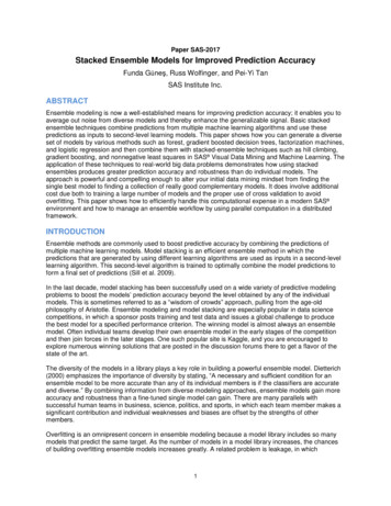
If an ID is selected more than once, the average prediction is used for each ID. After making sure that each ID is selected at least once in the 100 bootstrap samples of eachmodeling algorithm, mean OOF predictions are obtained by averaging over 100 bootstrap OOFpredictions. This simple averaging provided a significant reduction in the five-fold training ASE. Forexample, for the gradient boosting model, the five-fold training ASE of the best model (out of 100models) was 0.09351. When the OOF predictions of 100 gradient boosting models are averaged, thisvalue reduced to 0.09236.This approach produces four columns of OOF predictions (one for each of the four algorithms). Thesefour averaged models form the model library to be used in Level-3 stacking.For scoring on test data, the predictions from the 500 models, which are generated by the same learningalgorithm, are simply averaged.Figure 1 shows the five-fold cross validation and test average squared errors (ASEs, also often calledmean squared error, or MSE) of the four average models that form the model library to be used in Level-3stacking. The best performing single modeling method is the average gradient boosting model, which hasa five-fold cross validation ASE of 0.09236. It is best by a fairly significant margin according to the ASEperformance metric.Level-2 ModelsTraining ASETesting ASE(Five-Fold CV ASE)Average gradient boosting0.092360.09273Average forest0.096620.09665Average logistic regression0.104700.10370Average factorization machines0.111600.10930Figure 1. Five-Fold Cross Validation and Test ASEs of Models in the Model LibraryResults for Level 3With average OOF predictions in hand from Level 2, you are ready to build final ensembles and assessthe resulting models by using the test set predictions. The OOF predictions are stored in the SAS data settrain mean oofs, which includes four columns of OOF predictions for the four average models, an IDvariable, and the target variable. The corresponding test set is test mean preds which includes the samecolumns. The rest of the analyses in this paper use these two data sets, which are also available in theGitHub repository.Start a CAS Session and Load Data into CASThe following SAS code starts a CAS session and loads data into in the CAS in-memory distributedcomputing engine in the SAS Viya environment:/* Start a CAS session named mySession */cas mySession;/* Define a CAS engine libref for CAS in-memory data tables *//* Define a SAS libref for the directory that includes the data */libname cas sasioca;libname data "/folders/myfolders/";/* Load data into CAS using SAS DATA steps */data cas.train oofs;set data.train mean oofs;run;data cas.test preds;set data.test mean preds;run;7

REGRESSION STACKINGLet Y represent the target, X represent the space of inputs, and 𝑔1 , , 𝑔𝐿 denote the learned predictionsfrom L machine learning algorithms (for example, a set of out-of-fold predictions). For an interval target, alinear ensemble model builds a prediction function,𝑏(𝑔) 𝑤1 𝑔1 𝑤𝐿 𝑔𝐿where 𝑤𝑖 are the model weights. A simple way to specify these weights is to set them all equal to 1 𝐿 (asdone in Level-2) so that each model contributes equally to the final ensemble. You can alternativelyassign higher weight to models you think will perform better. For the Adult example, the gradient boostedtree OOF predictor is a natural candidate to weight higher because of its best single model performance.Although assigning weights by hand can often be reasonable, you can typically improve final ensembleperformance by using a learning algorithm to estimate them. Because of its computational efficiency andmodel interpretability, linear regression is a commonly used method for final model stacking. In aregression model that has an interval target, the model weights (𝑤𝑖 ) are found by solving the followingleast squares problem:𝑁𝑚𝑖𝑛 (𝑦𝑖 (𝑤1 𝑔1𝑖 𝑤𝐿 𝑔𝐿𝑖 ) )2𝑖 1REGULARIZATIONUsing cross validated predictions partially helps to deal with the overfitting problem. An attending difficultywith using OOF or OOB predictions as inputs is that they tend to be highly correlated with each other,creating the well-known collinearity problem for regression fitting. Arguably the best way to deal with thisproblem is to use some form of regularization for the model weights when training the highest-levelmodel. Regularization methods place one or more penalties on the objective function, based on the sizeof the model weights. If these penalty parameters are selected correctly, the total prediction error of themodel can decrease significantly and the parameters of the resulting model can be more stable.The following subsections illustrate a couple of good ways to regularize your ensemble model. Theyinvolve estimating and choosing one or more new hyperparameters that control the amount ofregularization. These hyperparameters can be determined by various methods, including a singlevalidation data partition, cross validation, and information criteria.Stacking with Adaptive LASSOConsider a linear regression of the following form:𝑏(𝑥) 𝑤1 𝑔1 𝑤𝐿 𝑔𝐿A LASSO learner finds the model weights by placing an 𝐿1 (sum of the absolute value of the weights)penalty on the model weights as follows:𝑁min (𝑦𝑖 (𝑤1 𝑔1𝑖 𝑤𝐿 𝑔𝐿𝑖 ) )2𝑖 1𝐿subject to 𝑤𝑖 𝑡𝑖 18

If the LASSO hyperparameter t is small enough, some of the weights will be exactly 0. Thus, the LASSOmethod produces a sparser and potentially more interpretable model. Adaptive LASSO (Zou 2006)modifies the LASSO penalty by applying adaptive weights (𝑣𝑗 ) to each parameter that forms the LASSOconstraint:𝐿subject to (𝑣𝑖 𝑤𝑖 ) 𝑡𝑖 1These constraints control shrinking the zero coefficients more than they control shrinking the nonzerocoefficients.The following REGSELECT procedure

set of models by various methods such as forest, gradient boosted decision trees, factorization machines, and logistic regression and then combine them with stacked-ensemble techniques such as hill climbing, gradient boosting, and nonnegative least squares in SAS Visual Data Mining and Machine Learning. The