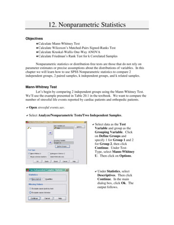
Transcription
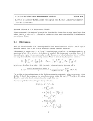
STAT 425: Introduction to Nonparametric StatisticsWinter 2018Lecture 6: Density Estimation: Histogram and Kernel Density EstimatorInstructor: Yen-Chi ChenReference: Section 6 of All of Nonparametric Statistics.Density estimation is the problem of reconstructing the probability density function using a set of given datapoints. Namely, we observe X1 , · · · , Xn and we want to recover the underlying probability density functiongenerating our dataset.6.1HistogramIf the goal is to estimate the PDF, then this problem is called density estimation, which is a central topic instatistical research. Here we will focus on the perhaps simplest approach: histogram.For simplicity, we assume that Xi [0, 1] so p(x) is non-zero only within [0, 1]. We also assume that p(x) issmooth and p0 (x) L for all x (i.e. the derivative is bounded). The histogram is to partition the set [0, 1](this region, the region with non-zero density, is called the support of a density function) into several binsand using the count of the bin as a density estimate. When we have M bins, this yields a partition: 1 2M 2 M 1M 11, B2 ,, · · · , BM 1 ,, BM ,1 .B1 0,MM MMMMIn such case, then for a given point x B , the density estimator from the histogram will bepbn (x) nnumber of observations within B 1MX I(Xi B ).nlength of the binn i 1The intuition of this density estimator is that the histogram assign equal density valuePnto every points withinthe bin. So for B that contains x, the ratio of observations within this bin is n1 i 1 I(Xi B ), whichshould be equal to the density estimate times the length of the bin.Now we study the bias of the histogram density estimator.E (bpn (x)) M · P (Xi B )Z M p(u)du M 1 M 1 M F FMM 1F M F M 1/M F M F 1M 1M M 1 p(x ), x ,.M M6-1
6-2Lecture 6: Density Estimation: Histogram and Kernel Density EstimatorThe last equality is done by the mean value theorem with F 0 (x) p(x). By the mean value theorem again,there exists another point x between x and x such thatp(x ) p(x) p0 (x ).x xThus, the biasbias(bpn (x)) E (bpn (x)) p(x) p(x ) p(x) p0 (x ) · (x x)(6.1) p0 (x ) · x x L .MNote that in the last inequality we use the fact that both x and x are within B , whose total length is 1/M ,so the x x 1/M . The analysis of the bias tells us that the more bins we are using, the less bias thehistogram has. This makes sense because when we have many bins, we have a higher resolution so we canapproximate the fine density structure better.Now we turn to the analysis of variance.!n1XI(Xi B )n i 1Var(bpn (x)) M 2 · Var M2 ·P (Xi B )(1 P (Xi B )).nBy the derivation in the bias, we know that P (Xi B ) Var(bpn (x)) M 2 ·p(x )Mp(x )M ,so the variance ) 1 p(xMnp(x ) p2 (x ) M· .nn(6.2)The analysis of the variance has an interesting result: the more bins we are using, the higher variance weare suffering.Now if we consider the MSE, the pattern will be more inspiring. The MSE isMSE(bpn (x)) bias2 (bpn (x)) Var(bpn (x)) L2p(x ) p2 (x ) . M·M2nn(6.3)An interesting feature of the histogram is that: we can choose M , the number of bins. When M is too large,the first quantity (bias) will be small while the second quantity (variance) will be large; this case is calledundersmoothing. When M is too small, the first quantity (bias) is large but the second quantity (variance)is small; this case is called oversmoothing.To balance the bias and variance, we choose M that minimizes the MSE, which leads to Mopt n · L2p(x ) 1/3.(6.4)Although in practice the quantity L and p(x ) are unknown so we cannot chose the optimal Mopt , the rule inequation (6.4) tells us how we should change the number of bins when we have more and more sample size.Practical rule of selecting M is related to the problem of bandwidth selection, a research topic in statistics.
Lecture 6: Density Estimation: Histogram and Kernel Density Estimator6.26-3Kernel Density Estimator0.000.010.02Density0.030.04Here we will talk about another approach–the kernel density estimator (KDE; sometimes called kernel densityestimation). The KDE is one of the most famous method for density estimation. The follow picture showsthe KDE and the histogram of the faithful dataset in R. The blue curve is the density curve estimated bythe KDE.405060708090100faithful waitingHere is the formal definition of the KDE. The KDE is a functionnpbn (x) 1 XKnh i 1 Xi xh ,(6.5)where K(x) is called the kernel function that is generally a smooth, symmetric function such as a Gaussianand h 0 is called the smoothing bandwidth that controls the amount of smoothing. Basically, the KDEsmoothes each data point Xi into a small density bumps and then sum all these small bumps together toobtain the final density estimate. The following is an example of the KDE and each small bump created byit:
Lecture 6: Density Estimation: Histogram and Kernel Density Estimator0.00.51.0Density1.56-4 0.20.00.20.40.60.81.0In the above picture, there are 6 data points located at where the black vertical segments indicate: 0.1, 0.2, 0.5, 0.7, 0.8, 0.15.The KDE first smooth each data point into a purple density bump and then sum them up to obtain the finaldensity estimate–the brown density curve.6.3Bandwidth and Kernel FunctionsThe smoothing bandwidth h plays a key role in the quality of KDE. Here is an example of applying differenth to the faithful dataset:0.000.010.02Density0.030.04h 1h 3h 10405060708090100faithful waitingClearly, we see that when h is too small (the green curve), there are many wiggly structures on our densitycurve. This is a signature of undersmoothing–the amount of smoothing is too small so that some structures
Lecture 6: Density Estimation: Histogram and Kernel Density Estimator6-5identified by our approach might be just caused by randomness. On the other hand, when h is too large (thebrown curve), we see that the two bumps are smoothed out. This situation is called oversmoothing–someimportant structures are obscured by the huge amount of smoothing.How about the choice of kernel function? A kernel function generally has two features:1. K(x) is symmetric.R2.K(x)dx 1.3. limx K(x) limx K(x) 0.In particular, the second requirement is needed to guarantee that the KDE pbn (x) is a probability densityfunction. Note that most kernel functions are positive; however, kernel functions could be negative 1 .In theory, the kernel function does not play a key role (later we will see this). But sometimes in practice,they do show some difference in the density estimator. In what follows, we consider three most commonkernel functions and apply them to the faithful dataset:01230.8 3 2 10123607080faithful waiting90100 101230.02Density0.010.020.000.010.0050 20.030.04Density0.030.040.03Density0.020.010.0040 30.04 10.05 20.05 echnikov Kernel1.0Uniform Kernel1.0Gaussian Kernel4050607080faithful waiting90100405060708090100faithful waitingThe top row displays the three kernel functions and the bottom row shows the corresponding density esti1 Some special types of kernel functions, known as the higher order kernel functions, will take negative value at some regions.These higher order kernel functions, though very counter intuitive, might have a smaller bias than the usual kernel functions.
6-6Lecture 6: Density Estimation: Histogram and Kernel Density Estimatormators. Here is the form of the three kernels:1 x2K(x) e 2 ,2π1Uniform K(x) I( 1 x 1),23Epanechnikov K(x) · max{1 x2 , 0}.4GaussianThe Epanechnikov is a special kernel that has the lowest (asymptotic) mean square error.Note that there are many many many other kernel functions such as triangular kernel, biweight kernel, cosinekernel, .etc. If you are interested in other kernel functions, please see https://en.wikipedia.org/wiki/Kernel (statistics).6.4Theory of the KDENow we will analyze the estimation error of the KDE. Assume that X1 , · · · , Xn are IID sample from anunknown density function p. In the density estimation problem, the parameter of interest is p, the truedensity function.To simplify the problem, assume that we focus on a given point x0 and we want to analyze the quality ofour estimator pbn (x0 ).Bias. We first analyze the bias. The bias of KDE is !nXi x01 XK p(x0 )E(bpn (x0 )) p(x0 ) Enh i 1h Xi x01 p(x0 ) E Khh Z1x x0 Kp(x)dx p(x0 ).hhNow we do a change of variable y ZE(bpn (x0 )) p(x0 ) x x0hKso that dy dx/h and the above becomesx x0h p(x)dx p(x0 )hZ K (y) p(x0 hy)dy p(x0 )(using the fact that x x0 hy).Now by Taylor expansion, when h is small,1p(x0 hy) p(x0 ) hy · p0 (x0 ) h2 y 2 p00 (x0 ) o(h2 ).2Note that o(h2 ) means that it is a smaller order term compared to h2 when h 0. Plugging this back to
Lecture 6: Density Estimation: Histogram and Kernel Density Estimator6-7the bias, we obtainZE(bpn (x0 )) p(x0 ) K (y) p(x0 hy)dy p(x0 ) 1 2 2 0020 K (y) p(x0 ) hy · p (x0 ) h y p (x0 ) o(h ) dy p(x0 )2ZZZ10 K (y) p(x0 )dy K (y) hy · p (x0 )dy K (y) h2 y 2 p00 (x0 )dy o(h2 ) p(x0 )2ZZZ1 p(x0 ) K (y) dy hp0 (x0 ) yK (y) dy h2 p00 (x0 ) y 2 K (y) dy o(h2 ) p(x0 )2{z} {z } 1 0Z1 2 002 p(x0 ) h p (x0 ) y K (y) dy p(x0 ) o(h2 )2Z1 2 00 h p (x0 ) y 2 K (y) dy o(h2 )21 h2 p00 (x0 )µK o(h2 ),2Zwhere µK Ry 2 K (y) dy. Namely, the bias of the KDE isbias(bpn (x0 )) 1 2 00h p (x0 )µK o(h2 ).2(6.6)This means that when we allow h 0, the bias is shrinking at a rate O(h2 ). Equation (6.6) reveals aninteresting fact: the bias of KDE is caused by the curvature (second derivative) of the density function!Namely, the bias will be very large at a point where the density function curves a lot (e.g., a very peakedbump). This makes sense because for such a structure, KDE tends to smooth it too much, making thedensity function smoother (less curved) than it used to be.Variance. For the analysis of variance, we can obtain an upper bound using a straight forward calculation: !n1 XXi x0Var(bpn (x0 )) VarKnh i 1h Xi x01Var K nh2h 1X x0i2 E Knh2h Z1x x02 Kp(x)dxnh2hZ10 K 2 (y)p(x0 hy)dy (using y x xand dy dx/h again)hnhZ1 K 2 (y) [p(x0 ) hyp0 (x0 ) o(h)] dynh Z12 p(x0 ) · K (y)dy o(h)nh Z112p(x0 ) K (y)dy o nhnh 112 p(x0 )σK o,nhnh
6-8Lecture 6: Density Estimation: Histogram and Kernel Density EstimatorR12where σK K 2 (y)dy. Therefore, the variance shrinks at rate O( nh) when n and h 0. Aninteresting fact from the variance is that: at point where the density value is large, the variance is also large!MSE. Now putting both bias and variance together, we obtain the MSE of the KDE:MSE(bpn (x0 )) bias2 (bpn (x0 )) Var(bpn (x0 ))112p(x0 )σK h4 p00 (x0 ) 2 µ2K o(h4 ) o4nh 14 O(h ) O.nh 1nh 12The first two term, 14 h4 p00 (x0 ) 2 µ2K nhp(x0 )σK, is called the asymptotic mean square error (AMSE). Inthe KDE, the smoothing bandwidth h is something we can choose. Thus, the bandwidth h minimizing theAMSE is 15214p(x0 ) σKhopt (x0 ) · C 1 · n 5 .n p00 (x0 ) 2 µ2KAnd this choice of smoothing bandwidth leads to a MSE at rate4MSEopt (bpn (x0 )) O(n 5 ).Remarks.4 The optimal MSE of the KDE is at rate O(n 5 ), which is faster than the optimal MSE of the histogram2O(n 3 )! However, both are slower than the MSE of a MLE (O(n 1 )). This reduction of error rate isthe price we have to pay for a more flexible model (we do not assume the data is from any particulardistribution but only assume the density function is smooth). In the above analysis, we only consider a single point x0 . In general, we want to control the overallMSE of the entire function. In this case, a straight forward generalization is the mean integrated squareerror (MISE): Z ZMISE(bpn ) E(bpn (x) p(x))2 MSE(bpn (x))dx.Under a similar derivation, one can show that ZZ1 411002224MISE(bpn ) h p (x) dxµK p(x)dx σK o(h ) o4nhnh {z } 1 Zµ2σ21 K · h4 · p00 (x) 2 dx K o(h4 ) o4nhnh {z}Overall curvature 1 O(h4 ) O.nh The two dominating terms in equation (6.7),µ2K44·h ·Z(6.7)σ2K p00 (x) 2 dx nh, is called the asymptotical mean {z}Overall curvatureintegrated square error (AMISE). The optimal smoothing bandwidth is often chosen by minimizing thisquantity. Namely, 512141σKhopt · R 00· 2 C 2 · n 5 .(6.8)2n p (x) dx µK
Lecture 6: Density Estimation: Histogram and Kernel Density Estimator6-9 However, the optimalR smoothing bandwidth hopt cannot be used in practice because it involves theunknown quantity p00 (x) 2 dx. Thus, how to choose h is an unsolved problem in statistics and isknown as bandwidth selection 2 . Most bandwidth selection approaches are either proposingRan estimateof AMISE and then minimizing the estimated AMISE or using an estimate of the curvature p00 (x) 2 dxand choose hopt accordingly.6.5Confidence Interval using the KDEIn this section, we will discuss an interesting topic–confidence interval of the KDE. For simplicity, we willfocus on the CI of the density function at a given point x0 . Recall from equation (6.5), nn1 XXi x01Xpbn (x0 ) K Yi ,nh i 1hn i 1where Yi h1 KXi x0h . Thus, the KDE evaluated at x0 is actually a sample mean of Y1 , · · · , Yn . By CLT, pbn (x0 ) E(bpn (x0 )) D N (0, 1).nVar(Yi )However, one has to be very careful when using this result because from the analysis of variance, Xi x01112K oVar(Yi ) Var p(x0 )σKhhhhdiverges when h 0. Thus, when h 0, the asymptotic distribution of pbn (x0 ) is D2nh (bpn (x0 ) E(bpn (x0 ))) N (0, p(x0 )σK).Thus, a 1 α CI can be constructed usingpbn (x0 ) z1 α/2 ·q2 .p(x0 )σKThis CI cannot be used in practice because p(x0 ) is unknown to us. One solution to this problem is toreplace it by the KDE, leading toq2 .pbn (x0 ) z1 α/2 · pbn (x0 )σKThere is another approach for constructing CIs called the bootstrap approach. However, this course is beyondthe scope of this course so we will not cover it here. If you are interested in it, you may take STAT 403 orcheck the lecture notes in the past: http://faculty.washington.edu/yenchic/17Sp stat403.html.Remarks. A problem of these CI is that the theoretical guarantee of coverage is for the expectation of the KDEE(bpn (x0 )) rather than the true density value p(x0 )! Recall from the analysis of bias, the bias is at theorder of O(h2 ). Thus, if h is fixed or h converges to 0 slowly, the coverage of CI will be lower than thenominal coverage (this is called undercoverage). Namely, even if we construct a 99% CI, the chancethat this CI covers the actual density value can be only 1% or even lower!In particular, when we choose h hopt , we always suffers from the problem of undercoverage becausethe bias and stochastic variation is at a similar order.2 Seehttps://en.wikipedia.org/wiki/Kernel density estimation#Bandwidth selection for more details.
6-10Lecture 6: Density Estimation: Histogram and Kernel Density Estimator To handle the problem of undercoverage, a most straight forward approach is to choose h 0 fasterthan the optimal rate. This method is called undersmoothing. However, when we undersmooth thedata, the MSE will be large (because the variance is going to get higher than the optimal case), meaningthat the accuracy of estimation decreases. Aside from the problem of bias, the CIs we construct are only for a single point x0 so the CI only hasa pointwise coverage. Namely, if we use the same procedure to construct a 1 α CI of every point,the probability that the entire density function is covered by the CI may be way less than the nominalconfidence level 1 α. There are approaches of constructing a CI such that it simultaneously covers the entire function. In thiscase, the CI will be called a confidence band because it is like a band with the nominal probability ofcovering the entire function. In general, how people construct a confidence band is via the bootstrap andthe band consists of two functions Lα (x), Uα (x) that can be constructed using the sample X1 , · · · , Xnsuch thatP (Lα (x) p(x) Uα (x) x) 1 α.6.6 Advanced Topics Other error measurements. In the above analysis, we focus on the MISE, which is related to theL2 error of estimating a function. In many theoretical analysis, researchers are often interested in Lqerrors: Z 1/qq bpn (x) p(x) dx.In particular, the L error, supx bpn (x) p(x) , is often used in many theoretical analysis. And theL error has an interesting error rate:!rlog n2,sup bpn (x) p(x) O(h ) OPnhx where the OP notation is a similar notation as O but is used for a random quantity. The extra log nterm has many interesting stories and it comes from the empirical process theory. We will learn partof this concept in the last few lectures. Derivative estimation. The KDE can also be used to estimate the derivative of a density function.For example, when we use the Gaussian kernel, the first derivative pb0n (x) is actually an estimator of thefirst derivative of true density p0 (x). Moreover, any higher order derivative can be estimated by thecorresponding derivatives of the KDE. The difference is, however, the MSE error rate will be different.If we consider estimating the -th derivative, p( ) , the MISE will be Z 1( )22MISE(bp( ) ) E(bp( )(x) p(x)) O(h) Onnh1 2 under suitableconditions. The bias generally remains at a similar rate but the variance is now at rate 1. Namely, the variance converges at a slower rate. The optimal MISE for estimating theO nh1 2 -th derivative of p will be 41MISEopt (bp( ) ) O n 5 2 , hopt, O(n 5 2 ).
Lecture 6: Density Estimation: Histogram and Kernel Density Estimator6-11 Multivariate density estimation. In addition to estimating the density function of a univariaterandom variable, the KDE can be applied to estimate the density function of a multivariate randomvariable. In this case, we need to use a multivariate kernel function. Generally, a multivariate kernelfunction can be constructed using a radial basis approach or a product kernel. Assume our data isd-dimensional. Let x (x1 , · · · , xd ) be the vector of each coordinate. The former uses cd · K (k xk)as the kernel function (cd is a constant depending on d, the dimension of the data). The later usesK( x) K(x1 )K(x2 ) · · · K(xd ) as the kernel function. In multivariate case, the KDE has a slowerconvergence rate: 411 MISEopt (bpn ) O n 4 d , hopt O n 4 d .MISE(bpn ) O(h4 ) OdnhHere you see that when d is large, the optimal convergence rate is very very slow. This means thatwe cannot estimate the density very well using the KDE when the dimension d of the data is large, aphenomenon known as the curse of dimensionality 3 .3 There are many forms of curse of dimensionality; the KDE is just one instance. For other cases, see https://en.wikipedia.org/wiki/Curse of dimensionality
The intuition of this density estimator is that the histogram assign equal density value to every points within the bin. So for B ' that contains x, the ratio of observations within this bin is 1 n P n i 1 I(X i 2B '), which should be equal to the density estimate times the length of the bin. Now we study the bias of the histogram density .
