Transcription
SDM’2010Columbus, OHOn the Power of Ensemble: Supervised andUnsupervised Methods Reconciled*Jing Gao1, Wei Fan2, Jiawei Han11 Department of Computer ScienceUniversity of Illinois2 IBM TJ Watson Research Center*Slides and references available athttp://ews.uiuc.edu/ jinggao3/sdm10ensemble.htm
Outline An overview of ensemble methods– Motivations– Tutorial overview Supervised ensemble Unsupervised ensemble Semi-supervised ensemble– Multi-view learning– Consensus maximization among supervised andunsupervised models Applications– Stream classification, transfer learning, anomalydetection2
Ensemblemodel 1DataEnsemble modelmodel 2 model kCombine multiplemodels into one!Applications: classification, clustering,collaborative filtering, anomaly detection 3
Stories of Success Million-dollar prize– Improve the baseline movierecommendation approach ofNetflix by 10% in accuracy– The top submissions all combineseveral teams and algorithms asan ensemble Data mining competitions– Classification problems– Winning teams employ anensemble of classifiers4
Netflix Prize Supervised learning task– Training data is a set of users and ratings (1,2,3,4,5stars) those users have given to movies.– Construct a classifier that given a user and anunrated movie, correctly classifies that movie aseither 1, 2, 3, 4, or 5 stars– 1 million prize for a 10% improvement over Netflix’scurrent movie recommender (MSE 0.9514) Competition– At first, single-model methods are developed, andperformances are improved– However, improvements slowed down– Later, individuals and teams merged their results,and significant improvements are observed5
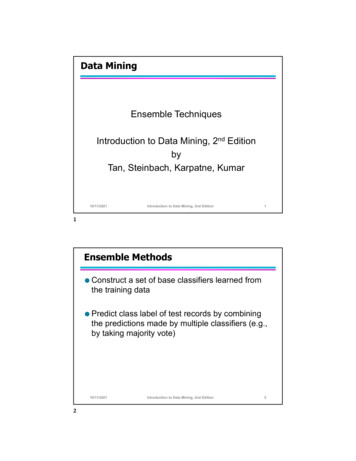
Leaderboard“Our final solution (RMSE 0.8712) consists of blending 107 individual results. “6
Motivations Motivations of ensemble methods– Ensemble model improves accuracy androbustness over single model methods– Applications: distributed computingprivacy-preserving applicationslarge-scale data with reusable modelsmultiple sources of data– Efficiency: a complex problem can bedecomposed into multiple sub-problems that areeasier to understand and solve (divide-andconquer approach)7
Relationship with Related Studies (1) Multi-task learning– Learn multiple tasks simultaneously– Ensemble methods: use multiple models to learn onetask Data integration– Integrate raw data– Ensemble methods: integrate information at the modellevel Mixture of models– Each model captures part of the global knowledge wherethe data have multi-modality– Ensemble methods: each model usually captures theglobal picture, but the models can complement eachother8
Relationship with Related Studies (2) Meta learning– Learn on meta-data (include base model output)– Ensemble methods: besides learn a joint modelbased on model output, we can also combine theoutput by consensus Non-redundant clustering– Give multiple non-redundant clustering solutionsto users– Ensemble methods: give one solution to userswhich represents the consensus among all thebase models9
Why Ensemble Works? (1) Intuition– combining diverse, independent opinions inhuman decision-making as a protectivemechanism (e.g. stock portfolio) Uncorrelated error reduction– Suppose we have 5 completely independentclassifiers for majority voting– If accuracy is 70% for each 10 (.7 3)(.3 2) 5(.7 4)(.3) (.7 5) 83.7% majority vote accuracy– 101 such classifiers 99.9% majority vote accuracyfrom T. Holloway, Introduction to EnsembleLearning, 2007.10
Why Ensemble Works? (2)Some unknown distributionModel 1Model 2Model 3Model 4Model 5Model 6Ensemble gives the global picture!11
Why Ensemble Works? (3) Overcome limitations of single hypothesis– The target function may not be implementable withindividual classifiers, but may be approximated by modelaveragingDecision TreeModel Averaging12
Research Focus Base models– Improve diversity! Combination scheme– Consensus (unsupervised)– Learn to combine (supervised) Tasks– Classification (supervised ensemble)– Clustering (unsupervised ensemble)13
SummarySupervisedLearningSVM,Logistic Regression, lective InferenceUnsupervisedLearningK-means,Spectral Clustering, .SingleModelsBoosting, ruleensemble, Bayesianmodel averaging, .Bagging, randomforest, randomdecision tree .Multi-view LearningConsensusMaximizationClustering EnsembleCombine bylearningCombine byconsensusReview the ensemblemethods in the tutorial14
Ensemble of Classifiers—Learn to Combinetrainingclassifier 1labeleddatatestEnsemble modelclassifier 2unlabeleddata classifier kfinalpredictionslearn the combination from labeled dataAlgorithms: boosting, stacked generalization, rule ensemble,Bayesian model averaging 15
Ensemble of Classifiers—Consensustrainingtestclassifier 1labeleddataclassifier 2unlabeleddatacombine thepredictions bymajority voting classifier kfinalpredictionsAlgorithms: bagging, random forest, random decision tree, modelaveraging of probabilities 16
Clustering Ensemble—Consensusclusteringalgorithm 1clusteringalgorithm 2 unlabeleddatacombine thepartitioningsby consensus clusteringalgorithm kAlgorithms: EM-based approach, instance-based, cluster-basedapproaches, correlation clustering, bipartite graph partitioningfinalclustering17
Semi-Supervised Ensemble—Learn to Combinetrainingtestclassifier 1labeleddataEnsemble modelunlabeleddataclassifier 2 classifier kfinalpredictionslearn the combination from bothlabeled and unlabeled dataAlgorithms: multi-view learning18
Semi-supervised Ensemble—Consensusclassifier 1labeleddataclassifier 2 classifier kclustering 1clustering hcombine all thesupervised andunsupervisedresults byconsensusfinalclustering 2 unlabeleddatapredictions Algorithms: consensus maximization19
Pros and ConsCombine bylearningCombine byconsensusProsGet useful feedbacks fromlabeled dataCan potentially improveaccuracyDo not need labeled dataCan improve the generalizationperformanceConsNeed to keep the labeleddata to train the ensembleMay overfit the labeled dataCannot work when nolabels are availableNo feedbacks from the labeleddataRequire the assumption thatconsensus is better20
Outline An overview of ensemble methods– Motivations– Tutorial overview Supervised ensemble Unsupervised ensemble Semi-supervised ensemble– Multi-view learning– Consensus maximization among supervised andunsupervised models Applications– Stream classification, transfer learning, anomalydetection21
Supervised Ensemble Methods Problem– Given a data set D {x1,x2, ,xn} and theircorresponding labels L {l1,l2, ,ln}– An ensemble approach computes: A set of classifiers {f1,f2, ,fk}, each of which mapsdata to a class label: fj(x) l A combination of classifiers f* which minimizesgeneralization error: f*(x) w1f1(x) w2f2(x) wkfk(x)22
Bias and Variance Ensemble methods– Combine weak learners to reduce variancefrom Elder, John. From Trees to Forests and Rule Sets - A UnifiedOverview of Ensemble Methods. 2007.23
Generating Base Classifiers Sampling training examples– Train k classifiers on k subsets drawn from the trainingset Using different learning models– Use all the training examples, but apply different learningalgorithms Sampling features– Train k classifiers on k subsets of features drawn fromthe feature space Learning ―randomly‖– Introduce randomness into learning procedures24
Bagging* (1) Bootstrap– Sampling with replacement– Contains around 63.2% original records in eachsample Bootstrap Aggregation– Train a classifier on each bootstrap sample– Use majority voting to determine the class labelof ensemble classifier*[Breiman96]25
Bagging (2)Bootstrap samples and classifiers:Combine predictions by majority votingfrom P. Tan et al. Introduction to Data Mining.26
Bagging (3) Error Reduction– Under mean squared error, bagging reduces varianceand leaves bias unchanged– Consider idealized bagging estimator: f ( x) E ( fˆz ( x))– The error isE[Y fˆz ( x)]2 E[Y f ( x) f ( x) fˆz ( x)]2 E[Y f ( x)]2 E[ f ( x) fˆ ( x)]2 E[Y f ( x)]2z– Bagging usually decreases MSEfrom Elder, John. From Trees to Forests and Rule Sets - A UnifiedOverview of Ensemble Methods. 2007.27
PrinciplesBoosting* (1)– Boost a set of weak learners to a strong learner– Make records currently misclassified more important Example– Record 4 is hard to classify– Its weight is increased, therefore it is more likelyto be chosen again in subsequent rounds*[FrSc97]from P. Tan et al. Introduction to Data Mining.28
Boosting (2) AdaBoost– Initially, set uniform weights on all the records– At each round Create a bootstrap sample based on the weights Train a classifier on the sample and apply it on the originaltraining set Records that are wrongly classified will have their weightsincreased Records that are classified correctly will have their weightsdecreased If the error rate is higher than 50%, start over– Final prediction is weighted average of all theclassifiers with weight representing the trainingaccuracy29
Boosting (3) Determine the weight– For classifier i, its error is i– The classifier’s importanceis represented as:j 1w j (Ci ( x j ) y j ) Nj 1wj1 1 i i ln 2 i w(ji 1) – The weight of each recordis updated as:– Final combination: Nw(ji ) exp i y j Ci ( x j ) Z (i )C ( x) arg max y i 1 i Ci ( x) y *K30
Classifications (colors) andWeights (size) after 1 iterationOf AdaBoost20 iterations3 iterationsfrom Elder, John. From Trees to Forestsand Rule Sets - A Unified Overview ofEnsemble Methods. 2007.31
Boosting (4) Explanation– Among the classifiers of the form:f ( x) i 1 i Ci ( x)K– We seek to minimize the exponential loss function: Nj 1exp y j f ( x j ) – Not robust in noisy settings32
Random Forests* (1) Algorithm–Choose T—number of trees to grow–Choose m M (M is the number of total features) —number of features used to calculate the best split ateach node–For each tree– Choose a training set by choosing N times (N is the number oftraining examples) with replacement from the training set For each node, randomly choose m features and calculate thebest split Fully grown and not prunedUse majority voting among all the trees*[Breiman01]33
Random Forests (2) Discussions– Bagging random features– Improve accuracy Incorporate more diversity and reduce variances– Improve efficiency Searching among subsets of features is much fasterthan searching among the complete set34
35
Random Decision Tree* (1) Principle–––Single-model learning algorithms Fix structure of the model, minimize some form of errors, or maximizedata likelihood (eg., Logistic regression, Naive Bayes, etc.) Use some ―free-form‖ functions to match the data given some―preference criteria‖ such as information gain, gini index and MDL. (eg.,Decision Tree, Rule-based Classifiers, etc.)Such methods will make mistakes if Data is insufficient Structure of the model or the preference criteria is inappropriate for theproblemEnsemble Make no assumption about the true model, neither parametric form norfree form Do not prefer one base model over the other, just average them*[FGM 05]36
Random Decision Tree (2) Algorithm–At each node, an un-used feature is chosen randomly ––A discrete feature is un-used if it has never been chosenpreviously on a given decision path starting from the root to thecurrent node.A continuous feature can be chosen multiple times on the samedecision path, but each time a different threshold value ischosenWe stop when one of the following happens: A node becomes too small ( 3 examples). Or the total height of the tree exceeds some limits, such as thetotal number of features.Prediction Simple averaging over multiple trees37
Random Decision Tree (3)B1: {0,1}B1 chosen randomlyB1 0B2: {0,1}B3: continuousB2: {0,1}YNRandomthreshold 0.3 B2: {0,1}B3 0.3?B2 0?B3: continuousB2 chosen randomlyY NB3: continuousB3 chosen randomlyRandom threshold 0.6B3 0.6?B3: continous38
Random Decision Tree (4) Potential Advantages– Training can be very efficient. Particularly truefor very large datasets. No cross-validation based estimation of parametersfor some parametric methods.– Natural multi-class probability.– Natural multi-label classification and probabilityestimation.– Imposes very little about the structures of themodel.39
Optimal Decision Boundaryfrom Tony Liu’s thesis (supervised by Kai Ming Ting)40
RDT lookslike the optimalboundary41
Outline An overview of ensemble methods– Motivations– Tutorial overview Supervised ensemble Unsupervised ensemble Semi-supervised ensemble– Multi-view learning– Consensus maximization among supervised andunsupervised models Applications– Stream classification, transfer learning, anomalydetection42
Clustering Ensemble Problem– Given an unlabeled data set D {x1,x2, ,xn}– An ensemble approach computes: A set of clustering solutions {C1,C2, ,Ck}, each ofwhich maps data to a cluster: fj(x) m A unified clustering solutions f* which combines baseclustering solutions by their consensus43
GoalMotivations– Combine ―weak‖ clusterings to a better onefrom A. Topchy et. al. ClusteringEnsembles: Models of Consensus andWeak Partitions. PAMI, 200544
Methods (1) How to get base models?– Bootstrap samples– Different subsets of features– Different clustering algorithms– Random number of clusters– Random initialization for K-means– Incorporating random noises into cluster labels– Varying the order of data in on-line methodssuch as BIRCH45
Methods (2) How to combine the models?– Direct approach Find the correspondence between the labels in thepartitions and fuse the clusters with the same labels– Indirect approach (Meta clustering) Treat each output as a categorical variable and clusterin the new feature space Avoid relabeling problems Algorithms differ in how they represent base modeloutput and how consensus is defined Focus on hard clustering methods in this tutorial46
An Examplebase clustering modelsobjectsthey may not represent The goal: get the consensus clusteringthe same cluster!47from A. Gionis et. al. Clustering Aggregation. TKDD, 2007
Cluster-based Similarity PartitioningAlgorithm (CSPA) Clustering objects– Similarity between two objects is defined as thepercentage of common clusters they fall into– Conduct clustering on the new similarity matrixSimilarity between vi and vj is: s (v , v ) Kk 1ij (Ck (vi ) Ck (v j ))K48
Cluster-based Similarity PartitioningAlgorithm (CSPA)v2v1v4v3v5v649
HyperGraph-Partitioning Algorithm (HGPA) Hypergraph representation and clustering– Each node denotes an object– A hyperedge is a generalization of an edge in that itcan connect any number of nodes– For objects that are put into the same cluster by aclustering algorithm, draw a hyperedge connectingthem– Partition the hypergraph by minimizing the numberof cut hyperedges– Each component forms a meta cluster50
HyperGraph-Partitioning Algorithm (HGPA)v2v1v4v3v5v6Hypergraph representation– acircle denotes a hyperedge51
Meta-Clustering Algorithm (MCLA) Clustering clusters– Regard each cluster from a base model as arecord– Similarity is defined as the percentage of sharedcommon objects eg. Jaccard measure– Conduct meta-clustering on these clusters– Assign an object to its most associated metacluster52
Meta-Clustering Algorithm g8g10M353
Comparisons* Time complexity– CSPA (clustering objects): O(n2kr)– HGPA (hypergraph partitioning): O(nkr)– MCLA (clustering clusters): O(nk2r2)– n-number of objects, k-number of clusters, rnumber of clustering solutions Clustering quality– MCLA tends to be best in low noise/diversitysettings– HGPA/CSPA tend to be better in highnoise/diversity settingsAll three algorithms are from *[StGh03]54
55
56
A Mixture Model of Consensus* Probability-based– Assume output comes from a mixture of models– Use EM algorithm to learn the model Generative model– The clustering solutions for each object arerepresented as nominal features--vi– vi is described by a mixture of k components, eachcomponent follows a multinomial distribution– Each component is characterized by distributionparameters j*[PTJ05]57
EM Method Maximize log likelihood ni 1 log j 1 j P(vi j )k Hidden variables– zi denotes which consensus cluster the objectbelongs to EM procedure– E-step: compute expectation of zi– M-step: update model parameters to maximizelikelihood58
59
60
Bipartite Graph Partitioning* Hybrid Bipartite Graph Formulation– Summarize base model output in a bipartitegraph– Lossless summarization—base model outputcan be reconstructed from the bipartite graph– Use spectral clustering algorithm to partition thebipartite graph– Time complexity O(nkr)—due to the specialstructure of the bipartite graph– Each component represents a consensus cluster*[FeBr04]61
Bipartite Graph sc7c8c9c10clusters62
Evaluation criterion:Normalized MutualInformation (NMI)Baseline methods:IBGF: clustering objectsCBGF: clustering clusters63
Summary of Unsupervised Ensemble Difference from supervised ensemble– No theories behind the success of clusteringensemble approaches– Moderate diversity is favored in the base modelsof clustering ensemble– There exist label correspondence problems Characteristics– Experimental results demonstrate that clusterensembles are better than single models!– There is no single, universally successful, clusterensemble method64
Outline An overview of ensemble methods– Motivations– Tutorial overview Supervised ensemble Unsupervised ensemble Semi-supervised ensemble– Multi-view learning– Consensus maximization among supervised andunsupervised models Applications– Stream classification, transfer learning, anomalydetection65
Multiple Source ClassificationImage Categorizationimages, descriptions,notes, comments,albums, tags .Like? Dislike?movie genres, cast,director, plots .users viewing history,movie ratings Research Areapublication and coauthorship network,published papers, .66
Model Combination helps!supervisedSupervised orunsupervisedTomSIGMODMaryVLDBAliceEDBTBobSome areas share similar keywordsPeople may publish in relevantCindyKDDbut different areasICDMTracySDMJackAAAIICMLThere may be crossdiscipline co-operationsMikeLucyJimunsupervised67
Multi-view Learning (1) Problem– The same set of objects can be described in multipledifferent views– Features are naturally separated into K sets:X ( X 1 , X 2 ,., X K )– Both labeled and unlabeled data are available– Learning on multiple views: Search for labeling on the unlabeled set and target functionson X: {f1,f2, ,fk} so that the target functions agree on labelingof unlabeled data68
Multi-view Learning (2) Conditions– Compatible --- all examples are labeled identically bythe target concepts in each view– Uncorrelated --- given the label of any example, itsdescriptions in each view are independent. Problems– Require raw data to learn the models– Supervised and unsupervised information sources aresymmetric Algorithms– Co-training69
InputCo-Training*– Features can be split into two sets: X X1 X 2– The two views are redundant but not completelycorrelated– Few labeled examples and relatively large amountsof unlabeled examples are available from the twoviews Intuitions– Two individual classifiers are learnt from the labeledexamples of the two views– The two classifiers’ predictions on unlabeledexamples are used to enlarge the size of training set– The algorithm searches for ―compatible‖ targetfunctions70*[BlMi98]
Labeled DataView 1Labeled DataView 2Classifier1Classifier2Unlabeled DataView 1Unlabeled DataView 171
72
Applications: Faculty WebpagesClassificationfrom S. K. Divvala. Co-Training & Its Applications in Vision.73
74
Outline An overview of ensemble methods– Motivations– Tutorial overview Supervised ensemble Unsupervised ensemble Semi-supervised ensemble– Multi-view learning– Consensus maximization among supervised andunsupervised models Applications– Stream classification, transfer learning, anomalydetection75
GoalConsensus Maximization*– Combine output of multiple supervised and unsupervisedmodels on a set of objects– The predicted labels should agree with the base modelsas much as possible Motivations– Unsupervised models provide useful constraints forclassification tasks– Model diversity improves prediction accuracy androbustness– Model combination at output level is needed due toprivacy-preserving or incompatible formats*[GLF 09]76
Problem77
A Toy 5x6x5x62x6x53x7x7x778
x42 79
Bipartite Graph[1 0 0][0 1 0][0 0 1]object i M1M2 qjgroup j ui conditional prob vectoradjacency 1 ui q jaij 0 otherwiseinitial probabilityM3M4 ui [ui1 ,., uic ] q j [q j1 ,., q jc ] GroupsObjects [1 0. 0] g j 1 y j . . [0 .0 1] g cj 80
Objective[1 0 0][0 1 0][0 0 1]minimize disagreement s 2 min Q,U ( aij ui q j q j y j 2 )nvi 1 j 1M1M2 qj uiSimilar conditional probability if theobject is connected to the group M3M4j 1Do not deviate much from the initialprobability GroupsObjects81
[1 0 0][0 1 0]Methodology[0 0 1]Iterate until convergence M1M2 qjUpdate probability of a group ui aij ui y j qj ai 1 qj i 1nij au ij inn i 1n ai 1ijUpdate probability of an object aq ij jv ui M3j 1v aj 1M4ij GroupsObjects82
Constrained Embeddingmin Q ,Ugroupsv qj 1 z 1au ancjzi 1nij izi 1ijq jz 1 if g j ' s label is zs 2 min Q,U ( aij ui q j q j y j 2 )nvi 1 j 1objectsj 1constraints for groups fromclassification models83
Ranking on Consensus Structure[1 0 0][0 1 0][0 0 1] 1 T 1q.1 D ( Dv A Dn A)q.1 D1 y.1 M1M2 qj ui qjqueryM3M4adjacencymatrixpersonalizeddamping factors GroupsObjects84
Incorporating Labeled Information[1 0 0] [0 1 0][0 0 1]Objective s 2 min Q,U ( aij ui q j q j y j 2 )nvi 1 j 1M1M2 qj 2 ui f i i 1 ui Update probability of a group auy ij i jn qj i 1n aiji 1M3M4j 1l au ij in qj i 1n ai 1ijUpdate probability of anv object aq ij jv ui GroupsObjectsj 1v aj 1ij ui aij q j fij 1v aj 1ij 85
Experiments-Data Sets 20 Newsgroup– newsgroup messages categorization– only text information available Cora– research paper area categorization– paper abstracts and citation information available DBLP– researchers area prediction– publication and co-authorship network, andpublication content– conferences’ areas are known86
Experiments-Baseline Methods (1) Single models– 20 Newsgroup: logistic regression, SVM, K-means, min-cut– Cora abstracts, citations (with or without a labeled set)– DBLP publication titles, links (with or without labels from conferences) Proposed method––––BGCMBGCM-L: semi-supervised version combining four models2-L: two models3-L: three models87
Experiments-Baseline Methods (2)SupervisedLearningSVM,Logistic Regression, lective InferenceUnsupervisedLearningK-means,Spectral Clustering, ng, .Mixture ofExperts,StackedGeneralizationMulti-view ing EnsembleEnsemble atRaw DataEnsembleat OutputLevel Ensemble approaches– clustering ensemble on all of the four modelsMCLA, HBGF88
Accuracy (1)89
Accuracy (2)90
Outline An overview of ensemble methods– Motivations– Tutorial overview Supervised ensemble Unsupervised ensemble Semi-supervised ensemble– Multi-view learning– Consensus maximization among supervised andunsupervised models Applications– Stream classification, transfer learning, anomalydetection91
Stream Classification* Process– Construct a classification model based on pastrecords– Use the model to predict labels for new data– Help decision ud92
Framework ClassificationModel ?Predict93
Existing Stream Mining Methods Shared distribution assumption– Training and test data are from the samedistribution P(x,y) x-feature vector, y-class label– Validity of existing work relies on the shareddistribution assumption Difference from traditional learning– Both distributions evolve training test 94
Evolving Distributions (1) An example of streamdata– KDDCUP’99 IntrusionDetection Data– P(y) evolves Shift or delay inevitable– The future data could be different from current data– Matching the current distribution to fit the future oneis a wrong way– The shared distribution assumption is inappropriate95
Evolving Distributions (2) Changes in P(y)– P(y) P(x,y) P(y x)P(x)– The change in P(y) is attributed to changes inP(y x) and P(x)TimeStamp 1TimeStamp 11TimeStamp 2196
Ensemble MethodC1f 1 ( x, y)f ( x, y) P(Y y x)f 2 ( x, y)C21 k if ( x, y ) f ( x, y)k i 1ETraining setTest set f k ( x, y)y x arg max y f E ( x, y)CkSimple Voting(SV) 1 model i predicts yf i ( x, y ) otherwise 0Averaging Probability(AP)f i ( x, y) probability of predicting y for model i97
Why it works? Ensemble– Reduce variance caused by single models– Is more robust than single models when thedistribution is evolving Simple averagingE– Simple averaging: uniform weights wi 1/k– Weighted ensemble: non-uniform weightskf ( x, y ) wi f i ( x, y )i 1 wi is inversely proportional to the training errors– wi should reflect P(M), the probability of model M after observingthe data– P(M) is changing and we could never estimate the true P(M) andwhen and how it changes– Uniform weights could minimize the expected distance betweenP(M) and weight vector98
An illustration Single models (M1, M2, M3) have huge variance. Simple averaging ensemble (AP) is more stable andaccurate. Weighted ensemble (WE) is not as Singlegood as AP sinceModelstraining errors and test errors may have verageTimeProbabilityStampATimeStampBTraining ErrorTest Error99
Experiments Set up– Data streams with chunks T1, T2, , TN– Use Ti as the training set to classify Ti 1 Measures– Mean Squared Error, Accuracy– Number of Wins, Number of Loses– Normalized Accuracy, MSE Methodsh( A, T ) h( A, T ) / max A (h( A, T ))– Single models: Decision tree (DT), SVM, Logistic Regression(LR)– Weighted ensemble: weights reflect the accuracy on training set(WE)– Simple ensemble: voting (SV) or probability averaging (AP)100
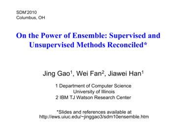
Experimental Results parison on Intrusion Data Set101
Experimental Results (3)Classification Accuracy Comparison102
Experimental Results (4)Mean Squared Error Comparison103
Outline An overview of ensemble methods– Motivations– Tutorial overview Supervised ensemble Unsupervised ensemble Semi-supervised ensemble– Multi-view learning– Consensus maximization among supervised andunsupervised models Applications– Stream classification, transfer learning, anomalydetection104
Standard Supervised New York Times85.5%New York Times105
In Reality training(labeled)test(unlabeled)ClassifierLabeled data notReutersavailable!New York Times64.1%New York Times106
Domain Difference Performance DroptrainNYTtestideal settingClassifierNew York TimesNYT85.5%New York Timesrealistic settingReutersReutersFrom Jing Jiang’s slidesClassifierNYT64.1%New York Times107
Other Examples Spam filtering– Public email collection personal inboxes Intrusion detection– Existing types of intrusions unknown types of intrusions Sentiment analysis– Expert review articles blog review articles The aim– To design learning methods that are aware of the training andtest domain difference Transfer learning– Adapt the classifiers learnt from the source domain to the newdomain108
All Sources of Labeled ed)Reuters ?ClassifierNew York TimesNewsgroup109
A Synthetic ExampleTrainingTest(have conflicting concepts) Partiallyoverlapping110
in To unify knowledge that are consistent with the testdomain from multiple source domains (models)111
Modified Bayesian Model AveragingBayesian Model AveragingModified for Transfer LearningM1M1M2 P ( M i D)Test setP( y x, M i )kMkP( y x) P( M i D) P( y x, M i )i 1M2 Test setP( y x, M i )P( M i x)Mk P( y x) k P( Mi 1i x) P( y x, M i )112
Global versus Local Weightsx2.40-2.69-3.972.085.081.43 5.230.55-3.62-3.732.154.48yM1wgwlM2wgwl100001 0.60.40.20.10.61 0.30.30.30.30.30.3 0.20.60.70.50.31 0.90.60.40.10.30.2 0.70.70.70.70.70.7 0.80.40.30.50.70 Locally weighting schemeTraining– Weight of each model is computed per example– Weights are determined according to models’performance on the test set, not training set113
Synthetic Example RevisitedM1M2TrainingTest(have conflicting concepts) Partiallyoverlapping114
Optimal Local WeightsHigher WeightC10.90.1Test example xC2H0.40.90.10.60.40.6w1w2w 0.80.80.2fk w ( x) 1i0.2i 1 Optimal weights– Solution to a regression problem– Impossible to get since f is unknown!115
Clustering-Manifold AssumptionTest examples that are closer infeature space are more likelyto share the same class label.116
Graph-based Heuristics Graph-based weights approximation– Map the structures of models onto test domainweighton xClusteringStructureM1M2117
Gr
an ensemble Data mining competitions -Classification problems -Winning teams employ an ensemble of classifiers. 5. Netflix Prize . the data have multi-modality -Ensemble methods: each model usually captures the globalpicture, but the models can complement each other . 9.