Transcription
Chapter 45ENSEMBLE METHODS FOR CLASSIFIERSLior RokachDepartment of Industrial EngineeringTel-Aviv Universityliorr@eng.tau.ac.ilAbstractThe idea of ensemble methodology is to build a predictive model by integrating multiple models. It is well-known that ensemble methods can be used forimproving prediction performance. In this chapter we provide an overview ofensemble methods in classification tasks. We present all important types ofensemble methods including boosting and bagging. Combining methods andmodeling issues such as ensemble diversity and ensemble size are discussed.Keywords:Ensemble, Boosting, AdaBoost, Windowing, Bagging, Grading, Arbiter Tree,Combiner Tree1.IntroductionThe main idea of ensemble methodology is to combine a set of models,each of which solves the same original task, in order to obtain a better composite global model, with more accurate and reliable estimates or decisionsthan can be obtained from using a single model. The idea of building a predictive model by integrating multiple models has been under investigation fora long time. Bühlmann and Yu (2003) pointed out that the history of ensemble methods starts as early as 1977 with Tukeys Twicing, an ensemble of twolinear regression models. Ensemble methods can be also used for improvingthe quality and robustness of clustering algorithms (Dimitriadou et al., 2003).Nevertheless, in this chapter we focus on classifier ensembles.In the past few years, experimental studies conducted by the machinelearning community show that combining the outputs of multiple classifiersreduces the generalization error (Domingos, 1996; Quinlan, 1996; Bauer andKohavi, 1999; Opitz and Maclin, 1999). Ensemble methods are very effective,mainly due to the phenomenon that various types of classifiers have differ-
958DATA MINING AND KNOWLEDGE DISCOVERY HANDBOOKent “inductive biases” (Geman et al., 1995; Mitchell, 1997). Indeed, ensemblemethods can effectively make use of such diversity to reduce the variance-error(Tumer and Ghosh, 1999; Ali and Pazzani, 1996) without increasing the biaserror. In certain situations, an ensemble can also reduce bias-error, as shownby the theory of large margin classifiers (Bartlett and Shawe-Taylor, 1998).The ensemble methodology is applicable in many fields such as: finance(Leigh et al., 2002), bioinformatics (Tan et al., 2003), healthcare (Mangiameliet al., 2004), manufacturing (Maimon and Rokach, 2004), geography (Bruzzone et al., 2004) etc.Given the potential usefulness of ensemble methods, it is not surprising thata vast number of methods is now available to researchers and practitioners.This chapter aims to organize all significant methods developed in this fieldinto a coherent and unified catalog. There are several factors that differentiatebetween the various ensembles methods. The main factors are:1. Inter-classifiers relationship — How does each classifier affect the otherclassifiers? The ensemble methods can be divided into two main types:sequential and concurrent.2. Combining method — The strategy of combining the classifiers generated by an induction algorithm. The simplest combiner determinesthe output solely from the outputs of the individual inducers. Ali andPazzani (1996) have compared several combination methods: uniformvoting, Bayesian combination, distribution summation and likelihoodcombination. Moreover, theoretical analysis has been developed for estimating the classification improvement (Tumer and Ghosh, 1999). Alongwith simple combiners there are other more sophisticated methods, suchas stacking (Wolpert, 1992) and arbitration (Chan and Stolfo, 1995).3. Diversity generator — In order to make the ensemble efficient, thereshould be some sort of diversity between the classifiers. Diversity maybe obtained through different presentations of the input data, as in bagging, variations in learner design, or by adding a penalty to the outputsto encourage diversity.4. Ensemble size — The number of classifiers in the ensemble.The following sections discuss and describe each one of these factors.2.Sequential MethodologyIn sequential approaches for learning ensembles, there is an interaction between the learning runs. Thus it is possible to take advantage of knowledgegenerated in previous iterations to guide the learning in the next iterations. We
Ensemble Methods For Classifiers959distinguish between two main approaches for sequential learning, as describedin the following sections (Provost and Kolluri, 1997).2.1Model-guided Instance SelectionIn this sequential approach, the classifiers that were constructed in previousiterations are used for manipulating the training set for the following iteration.One can embed this process within the basic learning algorithm. These methods, which are also known as constructive or conservative methods, usuallyignore all data instances on which their initial classifier is correct and onlylearn from misclassified instances.The following sections describe several methods which embed the sampleselection at each run of the learning algorithm.2.1.1Uncertainty Sampling.This method is useful in scenarios whereunlabeled data is plentiful and the labeling process is expensive. We can defineuncertainty sampling as an iterative process of manual labeling of examples,classifier fitting from those examples, and the use of the classifier to selectnew examples whose class membership is unclear (Lewis and Gale, 1994). Ateacher or an expert is asked to label unlabeled instances whose class membership is uncertain. The pseudo-code is described in Figure 45.1.Input: I (a method for building the classifier), b (the selected bulk size), U (aset on unlabled instances), E (an Expert capable to label instances)Output: C1: Xnew Random set of size b selected f rom U2: Ynew E(Xnew )3: S (Xnew , Ynew )4: C I(S)5: U U Xnew6: while E is willing to label instances do7:Xnew Select a subset of U of size b such that C is least certain of itsclassification.Ynew E(Xnew )8:9:S S (Xnew , Ynew )10:C I(S)11:U U Xnew12: end whileFigure 45.1.Pseudo-Code for Uncertainty Sampling.
960DATA MINING AND KNOWLEDGE DISCOVERY HANDBOOKIt has been shown that using uncertainty sampling method in text categorization tasks can reduce by a factor of up to 500 the amount of data that hadto be labeled to obtain a given accuracy level (Lewis and Gale, 1994).Simple uncertainty sampling requires the construction of many classifiers.The necessity of a cheap classifier now emerges. The cheap classifier selectsinstances “in the loop” and then uses those instances for training another, moreexpensive inducer. The Heterogeneous Uncertainty Sampling method achievesa given error rate by using a cheaper kind of classifier (both to build and run)which leads to reducted computational cost and run time (Lewis and Catlett,1994).Unfortunately, an uncertainty sampling tends to create a training set thatcontains a disproportionately large number of instances from rare classes. Inorder to balance this effect, a modified version of a C4.5 decision tree was developed (Lewis and Catlett, 1994). This algorithm accepts a parameter calledloss ratio (LR). The parameter specifies the relative cost of two types of errors: false positives (where negative instance is classified positive) and falsenegatives (where positive instance is classified negative). Choosing a loss ratio greater than 1 indicates that false positives errors are more costly than thefalse negative. Therefore, setting the LR above 1 will counterbalance the overrepresentation of positive instances. Choosing the exact value of LR requiressensitivity analysis of the effect of the specific value on the accuracy of theclassifier produced.The original C4.5 determines the class value in the leaves by checkingwhether the split decreases the error rate. The final class value is determinedby majority vote. In a modified C4.5, the leaf’s class is determined by comparison with a probability threshold of LR/(LR 1) (or its appropriate reciprocal).Lewis and Catlett (1994) show that their method leads to significantly higheraccuracy than in the case of using random samples ten times larger.2.1.2Boosting.Boosting (also known as arcing — Adaptive Resampling and Combining) is a general method for improving the performance ofany learning algorithm. The method works by repeatedly running a weaklearner (such as classification rules or decision trees), on various distributedtraining data. The classifiers produced by the weak learners are then combinedinto a single composite strong classifier in order to achieve a higher accuracythan the weak learner’s classifiers would have had.Schapire introduced the first boosting algorithm in 1990. In 1995 Freundand Schapire introduced the AdaBoost algorithm. The main idea of this algorithm is to assign a weight in each example in the training set. In the beginning,all weights are equal, but in every round, the weights of all misclassified instances are increased while the weights of correctly classified instances aredecreased. As a consequence, the weak learner is forced to focus on the diffi-
961Ensemble Methods For Classifierscult instances of the training set. This procedure provides a series of classifiersthat complement one another.The pseudo-code of the AdaBoost algorithm is described in Figure 45.2.The algorithm assumes that the training set consists of m instances, labeledas -1 or 1. The classification of a new instance is made by voting on allclassifiers {Ct }, each having a weight of αt . Mathematically, it can be writtenas:TXH(x) sign(αt · Ct (x))t 1Input: I (a weak inducer), T (the number of iterations), S (training set)Output: Ct , αt ; t 1, . . . , T1: t 12: D1 (i) 1/m; i 1, . . ., m3: repeat4:Build ClassifierCt using I and distribution DtP5:εt Dt (i)i:Ct (xi )6 yi6:7:8:9:10:11:12:13:14:if εt 0.5 thenT t 1exit Loop.end iftαt 12 ln( 1 εεt )Dt 1 (i) Dt (i) · e αt yt Ct (xi )Normalize Dt 1 to be a proper distribution.t until t TFigure 45.2.The AdaBoost Algorithm.The basic AdaBoost algorithm, described in Figure 45.2, deals with binaryclassification. Freund and Schapire (1996) describe two versions of the AdaBoost algorithm (AdaBoost.M1, AdaBoost.M2), which are equivalent for binary classification and differ in their handling of multiclass classification problems. Figure 45.3 describes the pseudo-code of AdaBoost.M1. The classification of a new instance is performed according to the following equation:H(x) argmax (Xy dom(y) t:C (x) ytlog1)βtAll boosting algorithms presented here assume that the weak inducers whichare provided can cope with weighted instances. If this is not the case, an
962DATA MINING AND KNOWLEDGE DISCOVERY HANDBOOKInput: I (a weak inducer), T (the number of iterations), S (the training set)Output: Ct , βt ; t 1, . . . , T1: t 12: D1 (i) 1/m; i 1, . . ., m3: repeat4:Build ClassifierCt using I and distribution DtPDt (i)5:εt i:Ct (xi )6 yi6:7:8:9:10:11:12:13:14:if εt 0.5 thenT t 1exit Loop.end ifεtβt 1 εt½βt Ct (xi ) yi1OtherwiseNormalize Dt 1 to be a proper distribution.t until t TDt 1 (i) Dt (i) ·Figure 45.3.The AdaBoost.M.1 Algorithm.unweighted dataset is generated from the weighted data by a resamplingtechnique. Namely, instances are chosen with probability according to theirweights (until the dataset becomes as large as the original training set).Boosting seems to improve performances for two main reasons:1. It generates a final classifier whose error on the training set is small bycombining many hypotheses whose error may be large.2. It produces a combined classifier whose variance is significantly lowerthan those produced by the weak learner.On the other hand, boosting sometimes leads to deterioration in generalizationperformance. According to Quinlan (1996) the main reason for boosting’sfailure is overfitting. The objective of boosting is to construct a compositeclassifier that performs well on the data, but a large number of iterations maycreate a very complex composite classifier, that is significantly less accuratethan a single classifier. A possible way to avoid overfitting is by keeping thenumber of iterations as small as possible.Another important drawback of boosting is that it is difficult to understand.The resulted ensemble is considered to be less comprehensible since the useris required to capture several classifiers instead of a single classifier. Despitethe above drawbacks, Breiman (1996) refers to the boosting idea as the mostsignificant development in classifier design of the nineties.
963Ensemble Methods For Classifiers2.1.3Windowing.Windowing is a general method aiming to improvethe efficiency of inducers by reducing the complexity of the problem. It wasinitially proposed as a supplement to the ID3 decision tree in order to addresscomplex classification tasks that might have exceeded the memory capacityof computers. Windowing is performed by using a sub-sampling procedure.The method may be summarized as follows: a random subset of the traininginstances is selected (a window). The subset is used for training a classifier,which is tested on the remaining training data. If the accuracy of the inducedclassifier is insufficient, the misclassified test instances are removed from thetest set and added to the training set of the next iteration. Quinlan (1993)mentions two different ways of forming a window: in the first, the currentwindow is extended up to some specified limit. In the second, several “key”instances in the current window are identified and the rest are replaced. Thusthe size of the window stays constant. The process continues until sufficientaccuracy is obtained, and the classifier constructed at the last iteration is chosenas the final classifier. Figure 45.4 presents the pseudo-code of the windowingprocedure.Input: I (an inducer), S (the training set), r (the initial window size), t (themaximum allowed windows size increase for sequential iterations).Output: C1: Window Select randomly r instances from S.2: Test S-Window3: repeat4:C I(W indow)5:Inc 06:for all (xi , yi ) T est do7:if C(xi ) 6 yi then8:T est T est (xi , yi )9:W indow W indow (xi , yi )10:Inc 11:end if12:if Inc t then13:exit Loop14:end ifend for15:16: until Inc 0Figure 45.4.The Windowing Procedure.The windowing method has been examined also for separate-and-conquerrule induction algorithms (Furnkranz, 1997). This research has shown thatfor this type of algorithm, significant improvement in efficiency is possible
964DATA MINING AND KNOWLEDGE DISCOVERY HANDBOOKin noise-free domains. Contrary to the basic windowing algorithm, this oneremoves all instances that have been classified by consistent rules from thiswindow, in addition to adding all instances that have been misclassified. Removal of instances from the window keeps its size small and thus decreasesinduction time.In conclusion, both windowing and uncertainty sampling build a sequenceof classifiers only for obtaining an ultimate sample. The difference betweenthem lies in the fact that in windowing the instances are labeled in advance,while in uncertainty, this is not so. Therefore, new training instances are chosen differently. Boosting also builds a sequence of classifiers, but combinesthem in order to gain knowledge from them all. Windowing and uncertaintysampling do not combine the classifiers, but use the best classifier.2.2Incremental Batch LearningIn this method the classifier produced in one iteration is given as “priorknowledge” to the learning algorithm in the following iteration (along with thesubsample of that iteration). The learning algorithm uses the current subsampleto evaluate the former classifier, and uses the former one for building the nextclassifier. The classifier constructed at the last iteration is chosen as the finalclassifier.3.Concurrent MethodologyIn the concurrent ensemble methodology, the original dataset is partitionedinto several subsets from which multiple classifiers are induced concurrently.The subsets created from the original training set may be disjoint (mutuallyexclusive) or overlapping. A combining procedure is then applied in order toproduce a single classification for a given instance. Since the method for combining the results of induced classifiers is usually independent of the inductionalgorithms, it can be used with different inducers at each subset. These concurrent methods aim either at improving the predictive power of classifiers ordecreasing the total execution time. The following sections describe severalalgorithms that implement this methodology.3.0.1Bagging.The most well-known method that processes samplesconcurrently is bagging (bootstrap aggregating). The method aims to improvethe accuracy by creating an improved composite classifier, I , by amalgamating the various outputs of learned classifiers into a single prediction.Figure 45.5 presents the pseudo-code of the bagging algorithm (Breiman,1996). Each classifier is trained on a sample of instances taken with replacement from the training set. Usually each sample size is equal to the size of theoriginal training set.
965Ensemble Methods For ClassifiersInput: I (an inducer), T (the number of iterations), S (the training set), N(the subsample size).Output: Ct ; t 1, . . . , T1: t 12: repeat3:St Sample N instances from S with replacment.4:Build classifier Ct using I on St5:t 6: until t TFigure 45.5.The Bagging Algorithm.Note that since sampling with replacement is used, some of the original instances of S may appear more than once in St and some may not be includedat all. So the training sets St are different from each other, but are certainly notindependent. To classify a new instance, each classifier returns the class prediction for the unknown instance. The composite bagged classifier, I , returnsthe class that has been predicted most often (voting method). The result is thatbagging produces a combined model that often performs better than the singlemodel built from the original single data. Breiman (1996) notes that this is trueespecially for unstable inducers because bagging can eliminate their instability. In this context, an inducer is considered unstable if perturbing the learningset can cause significant changes in the constructed classifier. However, thebagging method is rather hard to analyze and it is not easy to understand byintuition what are the factors and reasons for the improved decisions.Bagging, like boosting, is a technique for improving the accuracy of a classifier by producing different classifiers and combining multiple models. Theyboth use a kind of voting for classification in order to combine the outputs ofthe different classifiers of the same type. In boosting, unlike bagging, eachclassifier is influenced by the performance of those built before, so the newclassifier tries to pay more attention to errors that were made in the previousones and to their performances. In bagging, each instance is chosen with equalprobability, while in boosting, instances are chosen with probability proportional to their weight. Furthermore, according to Quinlan (1996), as mentionedabove, bagging requires that the learning system should not be stable, whereboosting does not preclude the use of unstable learning systems, provided thattheir error rate can be kept below 0.5.This procedure creates k classi3.0.2Cross-validated Committees.fiers by partitioning the training set into k-equal-sized sets and in turn, trainingon all but the i-th set. This method, first used by Gams (1989), employed 10fold partitioning. Parmanto et al. (1996) have also used this idea for creating an
966DATA MINING AND KNOWLEDGE DISCOVERY HANDBOOKensemble of neural networks. Domingos (1996) has used cross-validated committees to speed up his own rule induction algorithm RISE, whose complexityis O(n2 ), making it unsuitable for processing large databases. In this case,partitioning is applied by predetermining a maximum number of examples towhich the algorithm can be applied at once. The full training set is randomlydivided into approximately equal-sized partitions. RISE is then run on eachpartition separately. Each set of rules grown from the examples in partition pis tested on the examples in partition p 1, in order to reduce overfitting andimprove accuracy.4.Combining ClassifiersThe way of combining the classifiers may be divided into two main groups:simple multiple classifier combinations and meta-combiners. The simple combining methods are best suited for problems where the individual classifiersperform the same task and have comparable success. However, such combiners are more vulnerable to outliers and to unevenly performing classifiers.On the other hand, the meta-combiners are theoretically more powerful butare susceptible to all the problems associated with the added learning (such asover-fitting, long training time).4.1Simple Combining Methods4.1.1Uniform Voting.In this combining schema, each classifier hasthe same weight. A classification of an unlabeled instance is performed according to the class that obtains the highest number of votes. Mathematicallyit can be written as:XClass(x) argmax1ci dom(y) kci argmax P̂Mk (y cj x )cj dom(y)where Mk denotes classifier k and P̂Mk (y c x ) denotes the probability of yobtaining the value c given an instance x.This combining method was pre4.1.2Distribution Summation.sented by Clark and Boswell (1991). The idea is to sum up the conditionalprobability vector obtained from each classifier. The selected class is chosenaccording to the highest value in the total vector. Mathematically, it can bewritten as:XClass(x) argmaxP̂Mk (y ci x )ci dom(y) kThis combining method was investi4.1.3Bayesian Combination.gated by Buntine (1990). The idea is that the weight associated with each
967Ensemble Methods For Classifiersclassifier is the posterior probability of the classifier given the training set.XClass(x) argmaxP (Mk S ) · P̂Mk (y ci x )ci dom(y) kwhere P (Mk S ) denotes the probability that the classifier Mk is correct giventhe training set S. The estimation of P (Mk S ) depends on the classifier’srepresentation. Buntine (1990) demonstrates how to estimate this value fordecision trees.4.1.4Dempster–Shafer.The idea of using the Dempster–Shafer theory of evidence (Buchanan and Shortliffe, 1984) for combining models hasbeen suggested by Shilen (1990; 1992). This method uses the notion of basicprobability assignment defined for a certain class ci given the instance x: Y³1 P̂Mk (y ci x )bpa(ci , x) 1 kConsequently, the selected class is the one that maximizes the value of thebelief function:1bpa(ci , x)Bel(ci , x) ·A 1 bpa(ci , x)where A is a normalization factor defined as:Xbpa(ci , x)A 11 bpa(ci , x) ci dom(y)4.1.5Naı̈ve Bayes.Using Bayes’ rule, one can extend the Naı̈ve Bayesidea for combining various classifiers:class(x) Y P̂M (y cj x )kargmaxP̂ (y cj ) ·P̂ (y cj )cj dom(y)k 1P̂ (y cj ) 0The idea in this combining method is to4.1.6Entropy Weighting.give each classifier a weight that is inversely proportional to the entropy of itsclassification vector.XClass(x) argmaxEnt(Mk , x)ci dom(y)k:ci argmax P̂Mk (y cj x )cj dom(y)where:Ent(Mk , x) Xcj dom(y)³ P̂Mk (y cj x ) log P̂Mk (y cj x )
968DATA MINING AND KNOWLEDGE DISCOVERY HANDBOOK4.1.7Density-based Weighting .If the various classifiers were trainedusing datasets obtained from different regions of the instance space, it mightbe useful to weight the classifiers according to the probability of sampling xby classifier Mk , namely:XP̂Mk (x)Class(x) argmaxci dom(y)k:ci argmax P̂Mk (y cj x )cj dom(y)The estimation of P̂Mk (x) depend on the classifier representation and can notalways be estimated.4.1.8DEA Weighting Method.Recently there has been attempt to usethe DEA (Data Envelop Analysis) methodology (Charnes et al., 1978) in orderto assign weight to different classifiers (Sohn and Choi, 2001). They argue thatthe weights should not be specified based on a single performance measure,but on several performance measures. Because there is a trade-off among thevarious performance measures, the DEA is employed in order to figure out theset of efficient classifiers. In addition, DEA provides inefficient classifiers withthe benchmarking point.4.1.9Logarithmic Opinion Pool .According to the logarithmic opinion pool (Hansen, 2000) the selection of the preferred class is performed according to:PClass(x) argmax e kαk ·log(P̂Mk (y cj x ))cj dom(y)where αk denotes the weight of the k-th classifier, such that:Xαk 0;αk 14.1.10Order Statistics.Order statistics can be used to combine classifiers (Tumer and Ghosh, 2000). These combiners have the simplicity of asimple weighted combining method with the generality of meta-combiningmethods (see the following section). The robustness of this method is helpful when there are significant variations among classifiers in some part of theinstance space.4.2Meta-combining MethodsMeta-learning means learning from the classifiers produced by the inducersand from the classifications of these classifiers on training data. The followingsections describe the most well-known meta-combining methods.
Ensemble Methods For Classifiers9694.2.1Stacking .Stacking is a technique whose purpose is to achievethe highest generalization accuracy. By using a meta-learner, this method triesto induce which classifiers are reliable and which are not. Stacking is usuallyemployed to combine models built by different inducers. The idea is to create ameta-dataset containing a tuple for each tuple in the original dataset. However,instead of using the original input attributes, it uses the predicted classificationof the classifiers as the input attributes. The target attribute remains as in theoriginal training set.Test instance is first classified by each of the base classifiers. These classifications are fed into a meta-level training set from which a meta-classifier isproduced. This classifier combines the different predictions into a final one. Itis recommended that the original dataset will be partitioned into two subsets.The first subset is reserved to form the meta-dataset and the second subset isused to build the base-level classifiers. Consequently the meta-classifier predications reflect the true performance of base-level learning algorithms. Stackingperformances could be improved by using output probabilities for every classlabel from the base-level classifiers. In such cases, the number of input attributes in the meta-dataset is multiplied by the number of classes.Džeroski and Ženko (2004) have evaluated several algorithms for constructing ensembles of classifiers with stacking and show that the ensemble performs(at best) comparably to selecting the best classifier from the ensemble by crossvalidation. In order to improve the existing stacking approach, they proposeto employ a new multi-response model tree to learn at the meta-level and empirically showed that it performs better than existing stacking approaches andbetter than selecting the best classifier by cross-validation.4.2.2Arbiter Trees.This approach builds an arbiter tree in a bottomup fashion (Chan and Stolfo, 1993). Initially the training set is randomly partitioned into k disjoint subsets. The arbiter is induced from a pair of classifiersand recursively a new arbiter is induced from the output of two arbiters. Consequently for k classifiers, there are log2 (k) levels in the generated arbiter tree.The creation of the arbiter is performed as follows. For each pair of classifiers, the union of their training dataset is classified by the two classifiers. Aselection rule compares the classifications of the two classifiers and selects instances from the union set to form the training set for the arbiter. The arbiter isinduced from this set with the same learning algorithm used in the base level.The purpose of the arbiter is to provide an alternate classification when thebase classifiers present diverse classifications. This arbiter, together with anarbitration rule, decides on a final classification outcome, based upon the basepredictions. Figure 45.6 shows how the final classification is selected based onthe classification of two base classifiers and a single arbiter.
970DATA MINING AND KNOWLEDGE DISCOVERY HANDBOOKClassifier 1Classifier 2InstanceClassificationClassificationArbiterFigure sificationA Prediction from Two Base Classifiers and a Single Arbiter.The process of forming the union of data subsets; classifying it using a pairof arbiter trees; comparing the classifications; forming a training set; trainingthe arbiter; and picking one of the predictions, is recursively performed untilthe root arbiter is formed. Figure 45.7 illustrate an arbiter tree created fork 4. T1 T4 are the initial four training datasets from which four classifiersC1 C4 are generated concurrently. T12 and T34 are the training sets generatedby the rule selection from which arbiters are produced. A12 and A34 are thetwo arbiters. Similarly, T14 and A14 (root arbiter) are generated and the arbitertree is rsT1T2T3T4Data-subsetsFigure 45.7.Sample Arbiter Tree.Several schemes for arbiter trees were examined and differentiated fromeach other by the selection rule used. Here are three versions of rule selection:Only instances with classifications that disagree are chosen (group 1).Like group 1 defined above, plus instances that their classifications agreebut are incorrect (group 2).Like groups 1 and 2 defined above, plus instances that have the samecorrect classifications (group 3).
Ensemble Methods For Classifiers971Two versions of arbitration rules have been implemented; each one corresponds to the selection rule used for generating the training data at that level:For
ENSEMBLE METHODS FOR CLASSIFIERS Lior Rokach Department of Industrial Engineering Tel-Aviv University liorr@eng.tau.ac.il Abstract The idea of ensemble methodology is to build a predictive model by integrat-ing multiple models. It is well-known that ensemble methods can be used for . 960 DATA MINING AND KNOWLEDGE DISCOVERY HANDBOOK