Transcription
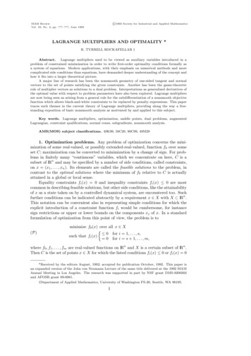
c 1993 Society for Industrial and Applied MathematicsSIAM ReviewVol. 35, No. 2, pp. ?–?, June 1993LAGRANGE MULTIPLIERS AND OPTIMALITY *R. TYRRELL ROCKAFELLAR †Abstract.Lagrange multipliers used to be viewed as auxiliary variables introduced in aproblem of constrained minimization in order to write first-order optimality conditions formally asa system of equations. Modern applications, with their emphasis on numerical methods and morecomplicated side conditions than equations, have demanded deeper understanding of the concept andhow it fits into a larger theoretical picture.A major line of research has been the nonsmooth geometry of one-sided tangent and normalvectors to the set of points satisfying the given constraints. Another has been the game-theoreticrole of multiplier vectors as solutions to a dual problem. Interpretations as generalized derivatives ofthe optimal value with respect to problem parameters have also been explored. Lagrange multipliersare now being seen as arising from a general rule for the subdifferentiation of a nonsmooth objectivefunction which allows black-and-white constraints to be replaced by penalty expressions. This papertraces such themes in the current theory of Lagrange multipliers, providing along the way a freestanding exposition of basic nonsmooth analysis as motivated by and applied to this subject.Key words. Lagrange multipliers, optimization, saddle points, dual problems, augmentedLagrangian, constraint qualifications, normal cones, subgradients, nonsmooth analysis.AMS(MOS) subject classifications. 49K99, 58C20, 90C99, 49M291. Optimization problems. Any problem of optimization concerns the minimization of some real-valued, or possibly extended-real-valued, function f0 over someset C; maximization can be converted to minimization by a change of sign. For problems in finitely many “continuous” variables, which we concentrate on here, C is asubset of lRn and may be specified by a number of side conditions, called constraints,on x (x1 , . . . , xn ). Its elements are called the feasible solutions to the problem, incontrast to the optimal solutions where the minimum of f0 relative to C is actuallyattained in a global or local sense.Equality constraints fi (x) 0 and inequality constraints fi (x) 0 are mostcommon in describing feasible solutions, but other side conditions, like the attainabilityof x as a state taken on by a controlled dynamical system, are encountered too. Suchfurther conditions can be indicated abstractly by a requirement x X with X lRn .This notation can be convenient also in representing simple conditions for which theexplicit introduction of a constraint function fi would be cumbersome, for instancesign restrictions or upper or lower bounds on the components xj of x. In a standardformulation of optimization from this point of view, the problem is to(P)minimize f0 (x) over all x X 0 for i 1, . . . , s,such that fi (x) 0 for i s 1, . . . , m,where f0 , f1 , . . . , fm are real-valued functions on lRn and X is a certain subset of lRn .Then C is the set of points x X for which the listed conditions fi (x) 0 or fi (x) 0*Received by the editors August, 1992; accepted for publication October, 1992. This paper isan expanded version of the John von Neumann Lecture of the same title delivered at the 1992 SIAMAnnual Meeting in Los Angeles. The research was supported in part by NSF grant DMS-9200303and AFOSR grant 89-0081.†Department of Applied Mathematics, University of Washington FS-20, Seattle, WA 98195.1
2r. t. rockafellarare satisfied. The presence of X can be suppressed by taking it to be all of lRn , whichwe refer to as the case of (P) where there’s no abstract constraint. In general it’scustomary to suppose—and for simplicity we’ll do so throughout this paper—that Xis closed, and that the objective function f0 and constraint functions fi are smooth(i.e., at least of class C 1 ).In classical problems of optimization, only equality constraints were seriouslyconsidered. Even today, mathematics is so identified with the study of “equations”that many people find it hard at first to appreciate the importance of inequalityconstraints and to recognize when they may be appropriate. Yet inequalities are thehallmark of modern optimization, affecting not just the scope of applications but thevery nature of the analysis that must be used. This is largely because of the computerrevolution, which has opened the way to huge problems of a prescriptive kind—wherethe goal may be to prescribe how some device should best be designed, or how somesystem should best be operated. In such problems in engineering, economics andmanagement, it’s typical that actions can be taken only within certain limited ranges,and that the consequences of the actions are desired to lie within certain other ranges.Clearly, inequality constraints are essential in representing such ranges.A set C specified as in (P) can be very complicated. Usually there’s no practicalway of decomposing C into a finite number of simple pieces which can be investigatedone by one. The process of minimizing f0 over C leads inevitably to the possibilitythat the points of interest may lie on the boundary of C. When inequality constraintscome into play, the geometry becomes one-sided and nontraditional forms of analysisare needed.A fundamental issue despite these complications is the characterization of the locally or globally optimal solutions to (P), if any. Not just any kind of characterizationwill do, however, in these days of diverse applications and exacting computationalrequirements. Conditions for optimality must not only be technically correct in theirdepiction of what’s necessary or sufficient, but rich in supplying information aboutpotential solutions and in suggesting a variety of numerical approaches. Moreoverthey should fit into a robust theoretical pattern which readily accommodates problemfeatures that might be elaborated beyond the statement so far in (P).Lagrange multipliers have long been used in optimality conditions involving constraints, and it’s interesting to see how their role has come to be understood frommany different angles. This paper aims at opening up such perspectives to the readerand providing an overview not only of the properties of Lagrange multipliers that canbe drawn upon in applications and numerical work, but also the new kind of analysisthat has needed to be developed. We’ll focus the discussion on first-order conditionsfor the most part, but this will already reveal differences in outlook and methodologythat distinguish optimization from other mathematical disciplines.One distinguishing idea which dominates many issues in optimization theory isconvexity. A set C lRn is said to be convex if it contains along with any two differentpoints the line segment joining those points:x C, x0 C, 0 t 1 (1 t)x tx0 C.(In particular, the empty set is convex, as are sets consisting of a single point.) Afunction f on lRn called convex if it satisfies the inequality f (1 t)x tx0 (1 t)f (x) tf (x0 ) for any x and x0 when 0 t 1.It’s concave if the opposite inequality always holds, and affine under equality; theaffine functions f : lRn lR have the form f (x) v·x const.
lagrange multipliers and optimality3Convexity is a large subject which can hardly be addressed here, see [1], but muchof the impetus for its growth in recent decades has come from applications in optimization. An important reason is the fact that when a convex function is minimizedover a convex set every locally optimal solution is global. Also, first-order necessaryconditions for optimality turn out to be sufficient. A variety of other properties conducive to computation and interpretation of solutions ride on convexity as well. Infact the great watershed in optimization isn’t between linearity and nonlinearity, butconvexity and nonconvexity. Even for problems that aren’t themselves of convex type,convexity may enter for instance in setting up subproblems as part of an iterativenumerical scheme.By the convex case of problem (P), we’ll mean the case where X is a convex setand, relative to X, the objective function f0 and the inequality constraint functionsf1 , . . . , fs are convex, and the equality constraints functions fs 1 , . . . , fm are affine.The feasible set C is then convex, so that a convex function is indeed being minimizedover a convex set. In such a problem the vectors of Lagrange multipliers that may beintroduced to express optimality have a remarkable significance. They generally solvean auxiliary problem of optimization which is dual to the given problem. Moreover, aswill be explained later, these two problems are the strategy problems associated withthe two players in a certain zero-sum game. Such game concepts have had a greatimpact on optimization, especially on its applications to areas like economics.Although we’re supposing in problem (P) that the fi ’s are smooth, it’s unavoidable that questions of nonsmooth analysis eventually be raised. In order to relateLagrange multipliers to perturbations of (P) with respect to certain canonical parameters, for instance, we’ll need to consider the optimal value (the minimum value of f0over C) as a function of such parameters, but this function can’t be expected to besmooth no matter how much smoothness is imposed on the fi ’s.Another source of nonsmoothness in optimization—there are many—is the frequent use of penalty expressions. Instead of solving problem (P) as stated, we maywish to minimize a function of the form f (x) f0 (x) ρ1 f1 (x) · · · ρm fm (x)(1.1)over the set X, where each ρi is a function on lR1 that gives the value 0 when fi (x)lies in the desired range, but some positive value (a penalty) when it lies outside thatrange. As an extreme case, infinite penalties might be used. Indeed, in taking 0if ui 0,for i 1, . . . , s :ρi (ui ) if ui 0, (1.2)0if ui 0,for i s 1, . . . , m : ρi (ui ) if ui 6 0,we get for f in (1.1) the so-called essential objective function in (P), whose minimization over X is equivalent to the minimization of f0 over C. Obviously, the essentialobjective function is far from smooth and even is discontinuous, but even finite penalties may be incompatible with smoothness. For example, linear penalty expressions 0if ui 0,for i 1, . . . , s :ρi (ui ) di uiif ui 0, (1.3)0if ui 0,for i s 1, . . . , m :ρi (ui ) di ui if ui 6 0,
4r. t. rockafellarwith positive constants di have “kinks” at the origin which prevent f from beingsmooth. Linear penalties have widely been used in numerical schemes since theirintroduction by Pietrzykowski [2] and Zangwill [3]. Quadratic penalty expressions 0if ui 0,for i 1, . . . , s :ρi (ui ) 12duifui 0,2 i i (1.4)0if ui 0,for i s 1, . . . , m :ρi (ui ) 12if ui 6 0,2 di uiwith coefficients di 0, first proposed in the inequality case by Courant [4], are firstorder smooth but discontinuous in their second derivatives. Penalty expressions witha possible mixture of linear and quadratic pieces have been suggested by Rockafellarand Wets [5], [6], [7], and Rockafellar [8] as offering advantages over the black-andwhite constraints in (1.2) even in the modeling of some situations, especially largescale problems with dynamic or stochastic structure. Similar expressions ρi have beenintroduced in connection with augmented Lagrangian theory, which will be describedin §6 and 7, but differing from penalty functions in the usual sense of that notionbecause they take on negative as well as positive values. Such “monitoring functions”nevertheless have the purpose of facilitating problem formulations in which standardconstraints are replaced by terms incorporated into a modified objective function,although at the possible expense of some nonsmoothness.For most of this paper we’ll keep to the conventional format of problem (P),but in §10 we’ll explain how the results can be extended to a more flexible problemstatement which covers the minimization of penalty expressions such as in (1.1) as wellas other nonsmooth objective functions that often arise in optimization modeling.2. The classical view. Lagrange multipliers first made their appearance inproblems having equality constraints only, which in the notation of (P) is the casewhere X lRn and s 0. The feasible set then has the form C x fi (x) 0 for i 1, . . . , m .(2.1)and can be approached geometrically as a “smooth manifold,” like an d-dimensionalhypersurface within lRn . This approach requires a rank assumption on the Jacobianmatrix of the mapping F : x 7 f1 (x), . . . , fm (x) from lRn into lRm . Specifically,if at a given point x̄ C the Jacobian matrix F (x̄) lRm n , whose rows are thegradient vectors fi (x̄), has full rank m, it’s possible to coordinatize C around x̄ soas to identify it locally with a region of lRd for d n m. The rank condition on F (x̄) is equivalent of course to the linear independence of the vectors fi (x̄) fori 1, . . . , m and entails having m n.The workhorse in this mathematical setting is the standard implicit mapping theorem along with its special case, the inverse mapping theorem. The linear independencecondition makes possible a local change of coordinates around x̄ which reduces theconstraints to an extremely simple form. Specifically, one can write x G(z), withx̄ G(z̄), for a smooth local mapping G having invertible Jacobian G(z̄), in such away that the transformed constraint functions hi fi G are just hi (z1 , . . . , zn ) ziand, therefore, the constraints on z (z1 , . . . , zn ) are just zi 0 for i 1, . . . , m.For the problem of minimizing the transformed objective function h0 f0 G subject to such constraints, there’s an elementary first-order necessary condition for theoptimality of z̄: one must have h0(z̄) 0 for i m 1, . . . , n. zi(2.2)
lagrange multipliers and optimality5A corresponding condition in the original coordinates can be stated in terms of thevalues h0ȳi (z̄) for i 1, . . . , m.(2.3) zi These have the property that h0 ȳ1 h1 · · · ȳm hm (z̄) 0, and this equationcan be written equivalently as f0 ȳ1 f1 · · · ȳm fm (x̄) 0.(2.4)Thus, a necessary condition for the local optimality of x̄ in the original problem is theexistence of values ȳi such that the latter holds.This result can be stated elegantly in terms of the Lagrangian for problem (P),which is the function L on lRn lRn defined byL(x, y) f0 (x) y1 f1 (x) · · · ym fm (x) for y (y1 , . . . , ym ).(2.5)Theorem 2.1. In the case of problem (P) where only equality constraints arepresent, if x̄ (x̄1 , . . . , x̄n ) is a locally optimal solution at which the gradients fi (x̄)are linearly independent, there must be a vector ȳ (ȳ1 , . . . , ȳm ) such that x L(x̄, ȳ) 0, y L(x̄, ȳ) 0.(2.6)The supplementary values ȳi in this first-order condition are called Lagrange multipliers for the constraint functions fi at x̄. An intriguing question is what they mightmean in a particular application, since it seems strange perhaps that a problem entirelyin lRn should require us to search for a vector pair in the larger space lRn lRm .The two equations in (2.6) can be combined into a single equation, the vanishingof the full gradient L(x̄, ȳ) relative to all the variables, but there’s a conceptualpitfall in this. The false impression is often gained that since the given problem in x isone of minimization, the vanishing of L(x̄, ȳ) should, at least in “nice” circumstanceswhen x̄ is optimal, correspond to L(x, y) achieving a local minimum with respect toboth x and y at (x̄, ȳ). But apart from the convex case of (P), L need not have a localminimum even with respect to x at x̄ when y is fixed at ȳ. On the other hand, it willbecome clear as we go along that the equation y L(x̄, ȳ) 0 should be interpretedon the basis of general principles as indicating a maximum of L with respect to y atȳ when x is fixed at x̄.The immediate appeal of (2.6) as a necessary condition for optimality resides inthe fact that these vector equations constitute n m scalar equations in the n munknowns x̄j and ȳi . The idea comes to mind that in solving the equations for x̄and ȳ jointly one may hope to determine some—or every—locally optimal solutionx̄ to (P). While this is definitely the role in which Lagrange multipliers were seentraditionally, the viewpoint is naive from current perspectives. The equations maywell be nonlinear. Solving a system of nonlinear equations numerically is no easierthan solving an optimization problem directly by numerical means. In fact, nonlinearequations are now often solved by optimization techniques through conversion to anonlinear least squares problem.Although a direct approach to the equality-constrained case of (P) through solving the equations in (2.6) may not be practical, Lagrange multipliers retain importancefor other reasons. Before delving into these, let’s look at the extent to which the classical methodology behind Theorem 2.1 is able to handle inequality constraints alongwith equality constraints.
6r. t. rockafellarAn inequality constraint fi (x) 0 is active at a point x̄ of the feasible set Cin (P ) if fi (x̄) 0, whereas it’s inactive if fi (x̄) 0. Obviously, in the theoreticalstudy of the local optimality of x̄ only the active inequality constraints at x̄ need tobe considered with the equality constraints, but as a practical matter it may be veryhard to know without a lot of computation exactly which of the inequality constraintsmight turn out to be active.As a temporary notational simplification, let’s suppose that the inequality constraints fi (x) 0 for i 1, . . . , r are inactive at x̄, whereas the ones for i r 1, . . . , sare active. (The set X is still the whole space lRn .) As long as all the gradients fi (x̄)for i r 1, . . . , s, s 1, . . . , m are linearly independent, we can follow the previouspattern of introducing a change of coordinates x G(z) such that the functionshi fi G take the form hi (z1 , . . . , zn ) zi for i r 1, . . . , m. Then the problem isreduced locally to minimizing h0 (z1 , . . . , zn ) subject to 0 for i r 1, . . . , s,zi 0 for i s 1, . . . , m.The former point x̄ is transformed into a point z̄ having coordinates z̄i 0 for i r 1, . . . , m. The elementary first-order necessary condition for the optimality of z̄ inthis setting is that h0 0 for i r 1, . . . , s,(z̄) 0 for i m 1, . . . , n. ziThen by lettingfor i 1, . . . , r, h0 (z̄) for i r 1, . . . , m, zi we obtain h0 ȳ1 h1 · · · ȳm hm (z̄) 0, which translates back to(0ȳi f0 ȳ1 f1 · · · ȳm fm (x̄) 0.This result can be stated as the following generalization of Theorem 2.1 in whichthe notation no longer supposes advance knowledge of the active set of inequalityconstraints.Theorem 2.2. In the case of problem (P) with both equality and inequality constraints possibly present, but no abstract constraint, if x̄ is a locally optimal solution atwhich the gradients fi (x̄) of the equality constraint functions and the active inequalityconstraint functions are linearly independent, there must be a vector ȳ in Y y (y1 , . . . , ys , ys 1 , . . . , ym ) yi 0 for i 1, . . . , s(2.7)such that x L(x̄, ȳ) 0, L 0 for i [1, s] with ȳi 0, and for i [s 1, m],(x̄, ȳ) 0 for i [1, s] with ȳi 0. yi(2.8)(2.9)The simple rule y L(x̄, ȳ) 0 in Theorem 2.1 has been replaced in Theorem 2.2by requirements imposed jointly on y L(x̄, ȳ) and ȳ. The significance of these complicated requirements will emerge later along with a more compact mode of expressingthem.
lagrange multipliers and optimality7Certainly Theorem 1.2 dispels further any illusion that the role of Lagrange multipliers is to enable an optimization problem to be solved by solving some systemof smooth nonlinear equations. Beyond the practical difficulties already mentioned,there’s now the fact that a whole collection of systems might be have to be inspected.For each subset I of {1, . . . , s} we could contemplate solving the n m equations L(x̄, ȳ) 0 for j 1, . . . , n, xj L(x̄, ȳ) 0 for i I and i s 1, . . . , m, yiȳi 0 for i {1, . . . , s} \ I,for the n m unknowns x̄j and ȳi and checking then to see whether the remainingconditions in Theorem 2.2, namely L(x̄, ȳ) 0 for i {1, . . . , s} \ I, yiȳi 0 for i I and i s 1, . . . , m,happen to be satisfied in addition. But the number of such systems to look at couldbe astronomical, so that an exhaustive search would be impossible.The first-order optimality conditions in Theorem 2.2 are commonly called theKuhn-Tucker conditions on the basis of the 1951 paper of Kuhn and Tucker [9], butafter many years it came to light that they had also been derived in the 1939 master’sthesis of Karush [10]. This thesis was never published, but the essential portions arereproduced in Kuhn’s 1976 historical account [11]. The very same theorem is provedby virtually the same approach in both cases, but with a “constraint qualification” interms of certain tangent vectors instead of the linear independence in Theorem 2.2.This will be explained in §4. Karush’s motivation came not from linear programming,an inspiring new subject when Kuhn and Tucker did their work, but from the calculusof variations. Others in the calculus of variations had earlier considered inequalityconstraints, for instance Valentine [12], but from a more limited outlook. Quite adifferent approach to inequality constraints, still arriving in effect at the same conditions, was taken before Kuhn and Tucker by John [13]. His hypothesis amountedto the generalization of the linear independence condition in Theorem 2.2 in whichthe coefficients of the gradients of the inequality constraint functions are restricted tononnegativity. This too will be explained in §4.Equality and inequality constraints are handled by Theorem 2.2, but not an abstract constraint x X. The optimality condition is therefore limited to applicationswhere it’s possible and convenient to represent all side conditions explicitly by a finite number of equations and inequalities. The insistence on linear independence ofconstraint gradients is a further shortcoming of Theorem 2.2. While the linear independence assumption is natural for equality constraints, it’s unnecessarily restrictivefor inequality constraints. It excludes many harmless situations that often arise, asfor instance when the constraints are merely linear (i.e., all the constraint functionsare affine) but the gradients are to some degree linearly dependent because of inherentsymmetries in the problem’s structure. This of course is why even the early contributors just cited felt the need for closer study of the constraint geometry in optimizationproblems.
8r. t. rockafellar3. Geometry of tangents and normals. The key to understanding Lagrangemultipliers has been the development of concepts pertinent to the minimization of afunction f0 over a set C lRn without insisting, at first, on any particular kind ofrepresentation for C. This not only furnishes insights for a variety of representationsof C, possibly involving an abstract constraint x X, but also leads to a better wayof writing multiplier conditions like the ones in Theorem 2.2.Proceeding for the time being under the bare assumption that C is some subsetof lRn , we discuss the local geometry of C in terms of “tangent vectors” and “normalvectors” at a point x̄. The introduction of such vectors in a one-sided sense, insteadof the classical two-sided manner, has been essential to advancement in optimizationtheory ever since inequality constraints came to the fore. It has stimulated the growthof a new branch of analysis, which is called nonsmooth analysis because of its emphasison one-sided derivative properties of functions as well as kinks and corners in setboundaries.Many different definitions of tangent and normal vectors have been offered overthe years. The systematic developments began with convex analysis in the 1960s andcontinued in the 70s and 80s with various extensions to nonconvex sets and functions.We take this opportunity to present current refinements which advantageously coverboth convex and nonconvex situations with a minimum of effort. The concepts willbe applied to Lagrange multipliers in §4.Definition 3.1. A vector w is tangent to C at x̄, written w TC (x̄), if thereis a sequence of vectors wk w along with a sequence of scalars tk 0 such thatx̄ tk wk C.Definition 3.2. A vector v is normal to C at x̄, written v NC (x̄), if there isa sequence of vectors v k v along with a sequence of points xk x̄ in C such that,for each k, v k , x xk o x xk for x C(3.1)(where h ·, ·i is the canonical inner product in lRn , · denotes the Euclidean norm,and o refers as usual to a term with the property that o(t)/t 0 as t 0). It is aregular normal vector if the sequences can be chosen constant, i.e., if actually v, x x̄ o x x̄ for x C.(3.2)Note that 0 TC (x̄), and whenever w TC (x̄) then also λw TC (x̄) for allλ 0. These properties also hold for NC (x̄) and mean that the sets TC (x̄) andNC (x̄) are cones in lRn . In the special case where C is a smooth manifold they turnout to be the usual tangent and normal subspaces to C at x̄, but in general theyaren’t symmetric about the origin: they may contain a vector without containing itsnegative. As subsets of lRn they’re always closed but not necessarily convex, althoughconvexity shows up very often.The limit process in Definition 3.2 introduces the set of pairs (x, v) with v anormal to C at x as the closure in C lRn of the set of pairs (x, v) with v a regularnormal to C at x. A basic consequencetherefore of Definition 3.2 is the following. Proposition 3.3. The set (x, v) v NC (x) is closed as a subset of C lRn :if xk x̄ in C and v k v with v k NC (xk ), then v NC (x̄).The symbols TC (x̄) and NC (x̄) are used to denote more than one kind of tangentcone and normal cone in the optimization literature. For the purposes here there isno need to get involved with a multiplicity of definitions and technical relationships,but some remarks may be helpful in providing orientation to other presentations ofthe subject.
lagrange multipliers and optimality9The cone we’re designating here by TC (x̄) was first considered by Bouligand [14],who called it the contingent cone to C at x̄. It was rediscovered early on in the studyof Lagrange multipliers for inequality constraints and ever since has been regarded asfundamental by everyone who has dealt with the subject, not only in mathematicalprogramming but control theory and other areas. For instance, Hestenes relied onthis cone in his 1966 book [15], which connected the then-new field of optimal controlwith the accomplishments of the 1930s school in the calculus of variations. Anotherimportant tangent cone is that of Clarke [16], which often agrees with TC (x̄) but ingeneral is a subcone of TC (x̄).The normal cone NC (x̄) coincides with the cone of “limiting normals” developedby Clarke [16], [17], [18] under the assumption that C is closed. (A blanket assumption of closedness would cause us trouble in §§8 and 9, so we avoid it here.) Clarkeused limits of more special “proximal” normals, instead of the regular normals v k inDefinition 3.2, but the cone comes out the same because every regular normal is itselfa limit of proximal normals when C is closed; cf. Kruger and Mordukhovich [19], orIoffe [20]). Clarke’s tangent cone consists of the vectors w such that hv, wi 0 for allv NC (x̄).Clarke was the first to take the crucial step of introducing limits to get a morerobust notion of normal vectors. But the normal cone really stressed by Clarke in [16],and well known now for its many successful applications to a diversity of problems,especially in optimal control and the calculus of variations (cf. [17] and [18]) isn’t thiscone of limit vectors, NC (x̄), but its closed convex hull.Clarke’s convexified normal cone and his tangent cone are polar to each other.For a long time such duality was felt to be essential in guiding the development ofnonsmooth analysis because of the experience that had been gained in convex analysis[1]. Although the cone of limiting normals was assigned a prominent role in Clarke’sframework, results in the calculus of normal vectors were typically stated in terms ofthe convexified normal cone, cf. Clarke [17] and Rockafellar [21]. This seemed a goodexpedient because (1) it promoted the desired duality, (2) in most of the examplesdeemed important at the time the cones turned out anyway to agree with the onesin Definitions 3.1 and 3.2, and (3) convexification was ultimately needed anyway incertain infinite-dimensional applications involving weak convergence. But gradually ithas become clear that convexification is an obstacle in some key areas, especially thetreatment of graphs of nonsmooth mappings.The move away from the convexifying of the cone of limiting normals has beenchampioned by Mordukhovich, who furnished the missing results needed to fill thecalculus gaps that had been feared in the absence of convexity [22], [23], [24]. Mordukhovich, like Clarke, emphasized “proximal” normals as the starting point for defining general normals through limits. The “regular” normals used here have not previously been featured in that expositional role, but they have long been familiar inoptimization under an alternative definition in terms of polarity with tangent vectors (the property in Proposition 3.5(b) below); cf. Bazaraa, Gould, and Nashed [25],Hestenes [26], Penot [27].Thanks to the efforts of many researchers, a streamlined theory is now in theoffing. Its outline will be presented here. We’ll be able to proceed on the basis o
Lagrange multipliers are now being seen as arising from a general rule for the subdifferentiation of a nonsmooth objective function which allows black-and-white constraints to be replaced by penalty expressions. This paper traces such themes in the current theory of Lagrange multipliers, providing along the way a free-