Transcription
lp.nb1Linear Programming,Lagrange Multipliers,and DualityGeoff Gordon
lp.nbOverviewThis is a tutorial about some interesting math and geometry connected withconstrained optimization. It is not primarily about algorithms—while itmentions one algorithm for linear programming, that algorithm is not new,and the math and geometry apply to other constrained optimizationalgorithms as well.The talk is organized around three increasingly sophisticated versions ofthe Lagrange multiplier theorem: the usual version, for optimizing smooth functions within smoothboundaries, an equivalent version based on saddle points, which we willgeneralize to the final version, for optimizing continuous functions over convexregions.Between the second and third versions, we will detour through thegeometry of convex cones.Finally, we will conclude with a practical example: a high-level descriptionof the log-barrier method for solving linear programs.2
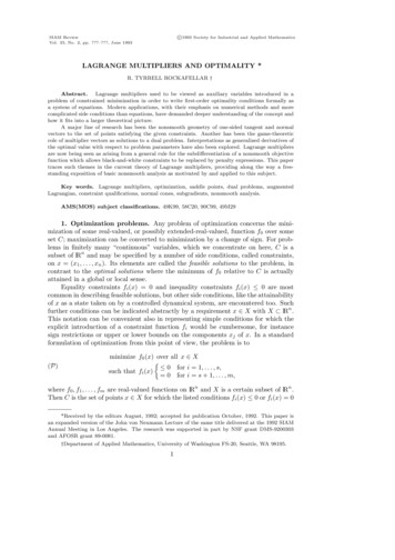
lp.nb3Lagrange MultipliersLagrange multipliers are a way to solve constrained optimization problems.For example, suppose we want to minimize the functionf Hx, yL x2 y2subject to the constraint0 gHx, yL x y - 2Here are the constraint surface, the contours of f , and the solution.
lp.nb4More Lagrange MultipliersNotice that, at the solution, the contours of f are tangent to the constraintsurface. The simplest version of the Lagrange Multiplier theorem saysthat this will always be the case for equality constraints: at theconstrained optimum, if it exists, “ f will be a multiple of “g.The Lagrange Multiplier theorem lets us translate the original constrainedoptimization problem into an ordinary system of simultaneous equationsat the cost of introducing an extra variable:gHx, yL 0“ f Hx, yL p “gHx, yLThe first equation states that x and y must satisfy the original constraint;the second equation adds the qualification that “ f and “g must beparallel. The new variable p is called a Lagrange multiplier.
lp.nb5The LagrangianWe can write this system of equations more compactly by defining theLagrangian L:LHx, y, pL f Hx, yL p gHx, yL x2 y2 pHx y - 2LThe equations are then just “ L 0, or in this casex y 22 x -p2 y -pThe unique solution for our example is x 1, y 1, p -2.
lp.nb6Multiple ConstraintsThe same technique allows us to solve problems with more than oneconstraint by introducing more than one Lagrange multiplier. Forexample, if we want to minimizex 2 y 2 z2subject tox y-2 0x z-2 0we can write the LagrangianLHx, y, z, p, qL x2 y2 z2 pHx y - 2L qHx z - 2Land the corresponding equations0 “x L 2 x p q0 “y L 2 y p0 “z L 2 z q0 “p L x y - 20 “q L x z - 2
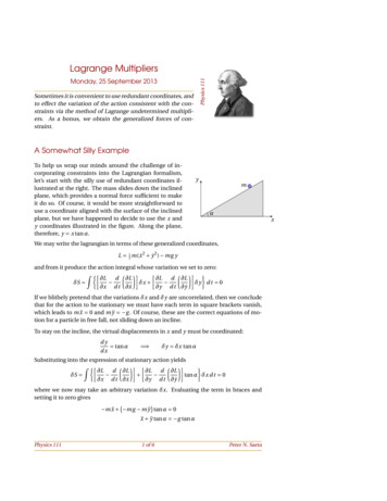
lp.nb7Multiple Constraints: the PictureThe solution to the above equations is9p Ø - ÅÅÅÅ4Å , q Ø - ÅÅÅÅ4Å , x Ø ÅÅÅÅ4Å , y Ø ÅÅÅÅ2Å , z Ø ÅÅÅÅ2Å 33333Here are the two constraints, together with a level surface of the objectivefunction. Neither constraint is tangent to the level surface; instead, thenormal to the level surface is a linear combination of the normals to thetwo constraint surfaces (with coefficients p and q).
lp.nb8Saddle PointsLagrange multiplier theorem, version 2: The solution, if it exists, isalways at a saddle point of the Lagrangian: no change in the originalvariables can decrease the Lagrangian, while no change in the multiplierscan increase it.For example, consider minimizing x2 subject to x 1. The Lagrangian isLHx, pL x2 pHx - 1L, which has a saddle point at x 1, p -2.32.521.5-11-1.5-200.5-2.51xp1.52-3pFor fixed p, L is a parabola with minimum at - ÅÅÅÅÅ (1 when p -2). For2fixed x, L is a line with slope x - 1 (0 when x 1).
lp.nb9Lagrangians as GamesBecause the constrained optimum always occurs at a saddle point of theLagrangian, we can view a constrained optimization problem as a gamebetween two players: one player controls the original variables and triesto minimize the Lagrangian, while the other controls the multipliers andtries to maximize the Lagrangian.If the constrained optimization problem is well-posed (that is, has a finiteand achievable minimum), the resulting game has a finite value (which isequal to the value of the Lagrangian at its saddle point).On the other hand, if the constraints are unsatisfiable, the player whocontrols the Lagrange multipliers can win (i.e., force the value to !),while if the objective function has no finite lower bound within theconstraint region, the player who controls the original variables can win(i.e., force the value to -!).We will not consider the case where the problem has a finite butunachievable infimum (e.g., minimize expHxL over the real line).
lp.nb10Inequality ConstraintsWhat if we want to minimize x2 y2 subject to x y - 2 0?We can use the same Lagrangian as before:LHx, y, pL x2 y2 pHx y - 2Lbut with the additional restriction that p § 0.Now, as long as x y - 2 0, the player who controls p can't doanything: making p more negative is disadvantageous, since it decreasesthe Lagrangian, while making p more positive is not allowed.Unfortunately, when we add inequality constraints, the simple condition“ L 0 is neither necessary nor sufficient to guarantee a solution to aconstrained optimization problem. (The optimum might occur at aboundary.)This is why we introduced the saddle-point version of the LM theorem.We can generalize the Lagrange multiplier theorem for inequalityconstraints, but we must use saddle points to do so.First, though, we need to look at the geometry of convex cones.
lp.nb11ConesIf g1 , g2 , . are vectors, the set 8 ai gi » ai 0 of all their nonnegativelinear combinations is a cone. The gi are the generators of the cone.The following picture shows two 2-dimensional cones which meet at theorigin. The dark lines bordering each cone form a minimal set ofgenerators for it; adding additional generating vectors from inside thecone wouldn't change the result.These particular two cones are duals of each other. The dual of a set C,written C¶ , is the set of all vectors which have a nonpositive dot productwith every vector in C. If C is a cone, then HC¶ L¶ C.
lp.nb12Special ConesAny set of vectors can generate a cone. The null set generates a conewhich contains only the origin; the dual of this cone is all of —n . Fewerthan n vectors generate a cone which is contained in a subspace of —n .If a cone contains both a (nonzero) vector and its negative, it is flat. Anylinear subspace of —n is an example of a flat cone. The following pictureshows another flat cone, along with its dual (which is not flat).A cone which is not flat is pointed. The dual of a full-rank flat cone is apointed cone which is not of full rank; the dual of a full-rank pointed coneis also a full-rank pointed cone.The dual of the positive orthant in —n is the negative orthant. If we reflectthe negative orthant around the origin, we get back the positive orthantagain. Cones with this property (that is, C -C¶ ) are called self-dual.
lp.nb13Faces and SuchWe have already seen the representation of a cone by its generators. Anyvector in the minimal set of generators for a cone is called an edge. (Theminimal set of generators is unique up to scaling.)Cones can also be represented by their faces, or bounding hyperplanes.Since each face must pass through the origin, we can describe a facecompletely by its normal vector.Conveniently, the face normals of any cone are the edges of its dual:
lp.nb14Representations of ConesAny linear transform of a cone is another cone. If we apply the matrix A(not necessarily square) to the cone generated by 8gi » i 1. . m , the resultis the cone generated by 8A gi » i 1. . m .In particular, if we write G for the matrix with columns gi , the cone Cgenerated by the gi is just the nonnegative orthant —m transformed by G.G is called the generating matrix for C. For example, the narrower of thetwo cones on the previous slide was generated by the matrixij 1 1 1 yzjjzjj 0 1 1 zzzjzk1 0 1{On the other hand, we sometimes have the bounding hyperplanes of Crather than its edges. That is, we have a matrix N whose columns are then face normals of C. In this case, N is the generating matrix of C¶ , andwe can write C as HN —n L¶ . The bounding-hyperplane representation ofour example cone isij -1 -1 1 yzjjzjj 1 0 -1 zzzjzk 1 1 -1 {Unfortunately, in higher dimensions it is difficult to translate betweenthese two representations of a cone. For example, finding the boundinghyperplanes of a cone from its generators is equivalent to finding theconvex hull of a set of points.
lp.nb15Convex Polytopes as ConesA convex polytope is a region formed by the intersection of some numberof halfspaces. A cone is also the intersection of halfspaces, with theadditional constraint that the halfspace boundaries must pass through theorigin. With the addition of an extra variable to represent the constantterm, we can represent any convex polytope as a cone: each edge of thecone corresponds to a vertex of the polytope, and each face of the conecorresponds to a face of the polytope.For example, to represent the 2D equilateral triangle with vertices atè!!!ij 1 yz jji 1 3k1{k 2yz ji 2zjè!!!{k1 3yzz{we add an extra coordinate (call it t) and write the triangle as theintersection of the plane t 1with the cone generated byè!!!ij 1 yz ijj 1 3jj zz jjjj 1 zz jj 2j zjk1{k 1yz ij 2zz jjzz jj 1 è!!!3zz jj{k 1yzzzzzzz{
lp.nb16Polytopes cont'dEquivalently, we can represent the same triangle by its boundinghyperplanes, one of which isij ÅÅÅÅ1Å I-3 è!!!3 M yz xjj 6zz ij yzjjzz jj zzjj ÅÅÅÅ1Å I-3 è!!!zz . jj y zz 03Mjj 6zz j zjjzz k 1 {1k{We can represent an unbounded polytope by allowing some of the cone’sedges not to intersect the plane t 1.
lp.nb17Geometric DualityThe idea of duality for cones is almost the same as the standard idea ofgeometric duality. A pair of dual cones represents a pair of dualpolytopes, with each vertex of one polytope corresponding to a face of theother and vice versa.Why almost: usually the geometric dual is thought of as insensitive tolocation and scaling, while the size and location of the polytoperepresented by the dual cone depend on the size of the original polytopeand its position relative to the origin. Also, strictly speaking, each conemust be the negative of the dual of the other, since by convention weintersect with the plane t 1 rather than t -1.
lp.nb18The Lagrange Multiplier TheoremWe can now state the Lagrange multiplier theorem in its most generalform, which tells how to minimize a function over an arbitrary convexpolytope N x c § 0.Lagrange multiplier theorem: The problem of finding x tominimize f HxLsubject to N x c § 0is equivalent to the problem of findingarg minx maxpe—n LHx, pLwhere the Lagrangian L is defined asLHx, pL f HxL pT HN x cLfor a vector of Lagrange multipliers p.The Lagrange multiplier theorem uses properties of convex cones andduality to transform our original problem (involving an arbitrarypolytope) to a problem which mentions only the very simple cone —n .(—n is simple for two reasons: it is axis-parallel, and it is self-dual.)The trade-offs are that we have introduced extra variables and that we arenow looking for a saddle point rather than a minimum.
lp.nb19Linear Programming DualityIf f HxL is a linear function (say f ' x) then the minimization problem is alinear program.The Lagrangian is f ' x p' HN x cL or, rearranging terms,H f ' p' NL x p' c.The latter is the Lagrangian for a new linear program (called the dualprogram):maximize p' csubject toN' p f 0p 0Since x was unrestricted in the original, or primal, program, it becomes avector of Lagrange multipliers for an equality constraint in the dualprogram.Note we minimize over x but maximize over p. (But changing § to changes p to - p.)
lp.nb20Duality cont'dEven though the primal and dual Lagrangians are the same, the primaland dual programs are not (quite) the same problem: in one, we wantmin p maxx L, in the other we want maxx min p L.It is a theorem (due to von Neumann) that these two values are the same(and so any x, p which achieves one also achieves the other).For nonlinear optimization problems, inf p supx L and supx inf p L are notnecessarily the same. The difference between the two is called a dualitygap.
lp.nb21Complementary SlacknessIf x, p is a saddle point of L, pT HN x cL § 0 (else LHx, 2 pL LHx, pL).Similarly, pT HN x cL 0 (else LIx, ÅÅÅÅ1Å pM LHx, pL).2So, pT HN x cL 0 (the complementary slackness condition).Since, in general, N x c will be zero in at most n coordinates, theremaining m - n components of p must be 0. (In fact, barring degeneracy,the constrained optimum will be at a vertex of the feasible region, soN x c will be zero in exactly n coordinates and p will have exactly nnonzeros.)
lp.nb22PricesSuppose x, p are a saddle point of f ' x p' HN x cL. How much does anincrease of d in fi change the value of the optimum?The value of the optimum increases by at least d xi , since the same x willstill be feasible (although perhaps not optimal).Similarly, a decrease of d in ci decreases the optimum by at least d pi .For this reason, dual variables are sometimes called shadow prices.
lp.nb23Log-barrier MethodsCommercial linear-programming solvers today use variants of thelogarithmic barrier method, a descendent of an algorithm introduced inthe 1980s by N. Karmarkar.Karmarkar's was the second polynomial-time algorithm to be discoveredfor linear programming, and the first practical one. (Khachiyan's ellipsoidalgorithm was the first, but in practice simplex seems to beat it.)We want to find a saddle point of L f ' x p' HN x cL with theconstraint p 0. Since even this simple constraint is inconvenient,consider what happens if we add an extra barrier term:L m f ' x p' HN x cL - m ln piThe effect of the barrier term is to make L m Ø ! as pi Ø 0, so that we canignore the constraints on p and work entirely with a smooth function. Therelative importance of the barrier term is controlled by the barrierparameter m 0.
lp.nb24Log-Barrier cont'dFor fixed x and m, L m is strictly convex, and so has a unique minimum.For fixed p and m, L m is linear.For each m, L m defines a saddle-point problem in x, p. For large m, theproblem is very smooth (and easy to solve); as m Ø 0, L m Ø L andHx* , p* Lm Ø x* , p* .Since L m is smooth, we can find the saddle point by setting “ L m 0 orN' p f 0N x c m p-1where p-1 means the componentwise inverse of p.The basic idea of the log-barrier method is to start with a large m andfollow the trajectory of solutions as m Ø 0. This trajectory is called thecentral path.
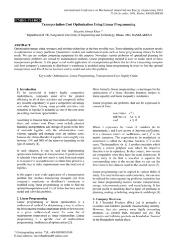
lp.nb25The Central PathHere is a portion of the central path for the problemminimize x ysubject tox 2y 1x, y 0This plot shows x, y as a function of m:21.510.50.511.52
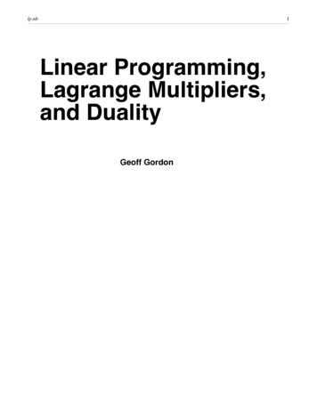
lp.nb26Central Path cont'dHere are the multipliers p, q, r . Note that p, q, r always satisfy theequality constraints of the dual problem, namely p r 1, q 2 r 1.0.40.200.40.30.60.7
lp.nb27Following the Central PathAgain, the optimality conditions are “ L m 0 orN' p f 0N x c m p-1If we start with a guess at x, p for a particular m, we can refine the guesswith one or more steps of Newton's method.After we're satisfied with the accuracy, we can decrease m and start again(using our previous solution as an initial guess). (One could—althoughwe won't—derive bounds on how close we need to be to the solutionbefore we can safely decrease m.)With the appropriate (nonobvious!) strategy for reducing m as much aspossible after each Newton step, we have a polynomial time algorithm.(In practice, we never use a provably-polynomial strategy since all theknown ones are very conservative.)
the Lagrange multiplier theorem: the usual version, for optimizing smooth functions within smooth boundaries, an equivalent version based on saddle points, which we will generalize to the final version, for optimizing continuous functions over convex regions. Between the second and third versions, we will detour through the