WIXLIB

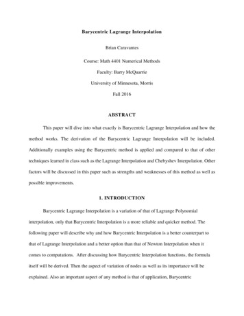
InterpolationPolynomial InterpolationPiecewise Polynomial InterpolationMonomial, Lagrange, and Newton InterpolationOrthogonal PolynomialsAccuracy and ConvergenceInterpolationPolynomial InterpolationPiecewise Polynomial InterpolationEvaluating PolynomialsMonomial, Lagrange, and Newton InterpolationOrthogonal PolynomialsAccuracy and ConvergenceLagrange InterpolationFor given set of data points (ti , yi ), i 1, . . . , n, Lagrangebasis functions are defined byWhen represented in monomial basis, polynomialn 1pn 1 (t) x1 x2 t · · · xn tcan be evaluated efficiently using Horner’s nestedevaluation scheme j (t) For example,(tj tk ),j 1, . . . , nk 1,k6 ji, j 1, . . . , nso matrix of linear system Ax y is identity matrix1 4t 5t2 2t3 3t4 1 t( 4 t(5 t( 2 3t)))Thus, Lagrange polynomial interpolating data points (ti , yi )is given byOther manipulations of interpolating polynomial, such asdifferentiation or integration, are also relatively easy withmonomial basis representationScientific ComputingnYFor Lagrange basis, 1 if i j j (ti ) ,0 if i 6 jwhich requires only n additions and n multiplicationsInterpolationPolynomial InterpolationPiecewise Polynomial Interpolation(t tk ) /k 1,k6 jpn 1 (t) x1 t(x2 t(x3 t(· · · (xn 1 txn ) · · · )))Michael T. HeathnYpn 1 (t) y1 1 (t) y2 2 (t) · · · yn n (t)17 / 56Michael T. HeathMonomial, Lagrange, and Newton InterpolationOrthogonal PolynomialsAccuracy and ConvergenceInterpolationPolynomial InterpolationPiecewise Polynomial InterpolationLagrange Basis FunctionsScientific Computing18 / 56Monomial, Lagrange, and Newton InterpolationOrthogonal PolynomialsAccuracy and ConvergenceExample: Lagrange InterpolationUse Lagrange interpolation to determine interpolatingpolynomial for three data points ( 2, 27), (0, 1), (1, 0)Lagrange polynomial of degree two interpolating threepoints (t1 , y1 ), (t2 , y2 ), (t3 , y3 ) is given by p2 (t) y1 interactive example (t t2 )(t t3 )(t t1 )(t t3 )(t t1 )(t t2 ) y2 y3(t1 t2 )(t1 t3 )(t2 t1 )(t2 t3 )(t3 t1 )(t3 t2 )For these particular data, this becomesLagrange interpolant is easy to determine but moreexpensive to evaluate for given argument, compared withmonomial basis representationp2 (t) 27t(t 1)(t 2)(t 1) ( 1)( 2)( 2 1)(2)( 1)Lagrangian form is also more difficult to differentiate,integrate, etc.Michael T. HeathInterpolationPolynomial InterpolationPiecewise Polynomial InterpolationScientific Computing19 / 56Monomial, Lagrange, and Newton InterpolationOrthogonal PolynomialsAccuracy and ConvergenceMichael T. HeathInterpolationPolynomial InterpolationPiecewise Polynomial InterpolationNewton InterpolationScientific Computing20 / 56Monomial, Lagrange, and Newton InterpolationOrthogonal PolynomialsAccuracy and ConvergenceNewton Basis FunctionsFor given set of data points (ti , yi ), i 1, . . . , n, Newtonbasis functions are defined byπj (t) j 1Y(t tk ),j 1, . . . , nk 1where value of product is taken to be 1 when limits make itvacuousNewton interpolating polynomial has formpn 1 (t) x1 x2 (t t1 ) x3 (t t1 )(t t2 ) interactive example · · · xn (t t1 )(t t2 ) · · · (t tn 1 )For i j, πj (ti ) 0, so basis matrix A is lower triangular,where aij πj (ti )Michael T. HeathInterpolationPolynomial InterpolationPiecewise Polynomial InterpolationScientific Computing21 / 56Monomial, Lagrange, and Newton InterpolationOrthogonal PolynomialsAccuracy and ConvergenceMichael T. HeathInterpolationPolynomial InterpolationPiecewise Polynomial InterpolationNewton Interpolation, continuedScientific Computing22 / 56Monomial, Lagrange, and Newton InterpolationOrthogonal PolynomialsAccuracy and ConvergenceExample: Newton InterpolationUse Newton interpolation to determine interpolatingpolynomial for three data points ( 2, 27), (0, 1), (1, 0)Using Newton basis, linear system is 100x1y1 1 t2 t1 x2 y2 01 t3 t1 (t3 t1 )(t3 t2 ) x3y3Solution x to system Ax y can be computed byforward-substitution in O(n2 ) arithmetic operationsMoreover, resulting interpolant can be evaluated efficientlyfor any argument by nested evaluation scheme similar toHorner’s methodFor these particular data, system is 1 0 0 x1 27 1 2 0 x2 1 1 3 3 x30Newton interpolation has better balance between cost ofcomputing interpolant and cost of evaluating itwhose solution by forward substitution is Tx 27 13 4 , so interpolating polynomial isp(t) 27 13(t 2) 4(t 2)tMichael T. HeathScientific Computing23 / 56Michael T. HeathScientific Computing24 / 56

InterpolationPolynomial InterpolationPiecewise Polynomial InterpolationMonomial, Lagrange, and Newton InterpolationOrthogonal PolynomialsAccuracy and ConvergenceInterpolationPolynomial InterpolationPiecewise Polynomial InterpolationNewton Interpolation, continuedDivided DifferencesIf pj (t) is polynomial of degree j 1 interpolating j givenpoints, then for any constant xj 1 ,Given data points (ti , yi ), i 1, . . . , n, divided differences,denoted by f [ ], are defined recursively bypj 1 (t) pj (t) xj 1 πj 1 (t)f [t1 , t2 , . . . , tk ] is polynomial of degree j that also interpolates same jpointsCoefficient of jth basis function in Newton interpolant isgiven byxj f [t1 , t2 , . . . , tj ]yj 1 pj (tj 1 ) πj 1 (tj 1 )Recursion requires O(n2 ) arithmetic operations to computecoefficients of Newton interpolant, but is less prone tooverflow or underflow than direct formation of triangularNewton basis matrixNewton interpolation begins with constant polynomialp1 (t) y1 interpolating first data point and thensuccessively incorporates each remaining data point intointerpolant interactive example Michael T. HeathScientific ComputingInterpolationPolynomial InterpolationPiecewise Polynomial Interpolationf [t2 , t3 , . . . , tk ] f [t1 , t2 , . . . , tk 1 ]tk t1where recursion begins with f [tk ] yk , k 1, . . . , nFree parameter xj 1 can then be chosen so that pj 1 (t)interpolates yj 1 ,xj 1Monomial, Lagrange, and Newton InterpolationOrthogonal PolynomialsAccuracy and Convergence25 / 56Monomial, Lagrange, and Newton InterpolationOrthogonal PolynomialsAccuracy and ConvergenceMichael T. HeathInterpolationPolynomial InterpolationPiecewise Polynomial InterpolationOrthogonal PolynomialsScientific Computing26 / 56Monomial, Lagrange, and Newton InterpolationOrthogonal PolynomialsAccuracy and ConvergenceOrthogonal Polynomials, continuedInner product can be defined on space of polynomials oninterval [a, b] by takingZ bhp, qi p(t)q(t)w(t)dtFor example, with inner product given by weight functionw(t) 1 on interval [ 1, 1], applying Gram-Schmidtprocess to set of monomials 1, t, t2 , t3 , . . . yields Legendrepolynomialsawhere w(t) is nonnegative weight function1, t, (3t2 1)/2, (5t3 3t)/2, (35t4 30t2 3)/8,Two polynomials p and q are orthogonal if hp, qi 0(63t5 70t3 15t)/8, . . .Set of polynomials {pi } is orthonormal if 1 if i jhpi , pj i 0 otherwisefirst n of which form an orthogonal basis for space ofpolynomials of degree at most n 1Other choices of weight functions and intervals yield otherorthogonal polynomials, such as Chebyshev, Jacobi,Laguerre, and HermiteGiven set of polynomials, Gram-Schmidt orthogonalizationcan be used to generate orthonormal set spanning samespaceMichael T. HeathInterpolationPolynomial InterpolationPiecewise Polynomial InterpolationScientific Computing27 / 56Monomial, Lagrange, and Newton InterpolationOrthogonal PolynomialsAccuracy and ConvergenceInterpolationPolynomial InterpolationPiecewise Polynomial InterpolationOrthogonal Polynomials, continuedare orthogonal with respect to weight function (1 t2 ) 1/2pk 1 (t) (αk t βk )pk (t) γk pk 1 (t)First few Chebyshev polynomials are given bywhich makes them very efficient to generate and evaluate1, t, 2t2 1, 4t3 3t, 8t4 8t2 1, 16t5 20t3 5t, . . .Orthogonality makes them very natural for least squaresapproximation, and they are also useful for generatingGaussian quadrature rules, which we will see laterScientific Computing28 / 56Monomial, Lagrange, and Newton InterpolationOrthogonal PolynomialsAccuracy and Convergencekth Chebyshev polynomial of first kind, defined on interval[ 1, 1] byTk (t) cos(k arccos(t))They satisfy three-term recurrence relation of formInterpolationPolynomial InterpolationPiecewise Polynomial InterpolationScientific ComputingChebyshev PolynomialsOrthogonal polynomials have many useful propertiesMichael T. HeathMichael T. HeathEqui-oscillation property : successive extrema of Tk areequal in magnitude and alternate in sign, which distributeserror uniformly when approximating arbitrary continuousfunction29 / 56Monomial, Lagrange, and Newton InterpolationOrthogonal PolynomialsAccuracy and ConvergenceMichael T. HeathInterpolationPolynomial InterpolationPiecewise Polynomial InterpolationChebyshev Basis FunctionsScientific Computing30 / 56Monomial, Lagrange, and Newton InterpolationOrthogonal PolynomialsAccuracy and ConvergenceChebyshev PointsChebyshev points are zeros of Tk , given by (2i 1)πti cos, i 1, . . . , k2kor extrema of Tk , given by iπti cos,ki 0, 1, . . . , kChebyshev points are abscissas of points equally spacedaround unit circle in R2 interactive example Chebyshev points have attractive properties forinterpolation and other problemsMichael T. HeathScientific Computing31 / 56Michael T. HeathScientific Computing32 / 56

InterpolationPolynomial InterpolationPiecewise Polynomial InterpolationMonomial, Lagrange, and Newton InterpolationOrthogonal PolynomialsAccuracy and ConvergenceInterpolationPolynomial InterpolationPiecewise Polynomial InterpolationInterpolating Continuous FunctionsMonomial, Lagrange, and Newton InterpolationOrthogonal PolynomialsAccuracy and ConvergenceInterpolating Continuous Functions, continuedIf data points are discrete sample of continuous function,how well does interpolant approximate that functionbetween sample points?If f (n) (t) M for all t [t1 , tn ], andh max{ti 1 ti : i 1, . . . , n 1}, thenIf f is smooth function, and pn 1 is polynomial of degree atmost n 1 interpolating f at n points t1 , . . . , tn , thenmax f (t) pn 1 (t) t [t1 ,tn ]f (n) (θ)f (t) pn 1 (t) (t t1 )(t t2 ) · · · (t tn )n!M hn4nError diminishes with increasing n and decreasing h, butonly if f (n) (t) does not grow too rapidly with nwhere θ is some (unknown) point in interval [t1 , tn ] interactive example Since point θ is unknown, this result is not particularlyuseful unless bound on appropriate derivative of f isknownMichael T. HeathScientific ComputingInterpolationPolynomial InterpolationPiecewise Polynomial Interpolation33 / 56Monomial, Lagrange, and Newton InterpolationOrthogonal PolynomialsAccuracy and ConvergenceMichael T. HeathInterpolationPolynomial InterpolationPiecewise Polynomial InterpolationHigh-Degree Polynomial InterpolationScientific ComputingConvergenceInterpolating polynomials of high degree are expensive todetermine and evaluatePolynomial interpolating continuous function may notconverge to function as number of data points andpolynomial degree increasesIn some bases, coefficients of polynomial may be poorlydetermined due to ill-conditioning of linear system to besolvedEqually spaced interpolation points often yieldunsatisfactory results near ends of intervalHigh-degree polynomial necessarily has lots of “wiggles,”which may bear no relation to data to be fitIf points are bunched near ends of interval, moresatisfactory results are likely to be obtained withpolynomial interpolationPolynomial passes through required data points, but it mayoscillate wildly between data pointsMichael T. HeathScientific ComputingInterpolationPolynomial InterpolationPiecewise Polynomial InterpolationUse of Chebyshev points distributes error evenly andyields convergence throughout interval for any sufficientlysmooth function35 / 56Monomial, Lagrange, and Newton InterpolationOrthogonal PolynomialsAccuracy and ConvergenceScientific Computing36 / 56Monomial, Lagrange, and Newton InterpolationOrthogonal PolynomialsAccuracy and ConvergenceExample: Runge’s FunctionPolynomial interpolants of Runge’s function at equallyspaced points do not convergePolynomial interpolants of Runge’s function at Chebyshevpoints do converge interactive example interactive example InterpolationPolynomial InterpolationPiecewise Polynomial InterpolationMichael T. HeathInterpolationPolynomial InterpolationPiecewise Polynomial InterpolationExample: Runge’s FunctionMichael T. Heath34 / 56Monomial, Lagrange, and Newton InterpolationOrthogonal PolynomialsAccuracy and ConvergenceScientific Computing37 / 56Monomial, Lagrange, and Newton InterpolationOrthogonal PolynomialsAccuracy and ConvergenceMichael T. HeathInterpolationPolynomial InterpolationPiecewise Polynomial InterpolationTaylor PolynomialScientific Computing38 / 56Piecewise Polynomial InterpolationHermite Cubic InterpolationCubic Spline InterpolationPiecewise Polynomial InterpolationFitting single polynomial to large number of data points islikely to yield unsatisfactory oscillating behavior ininterpolantAnother useful form of polynomial interpolation for smoothfunction f is polynomial given by truncated Taylor seriespn (t) f (a) f 0 (a)(t a) f 00 (a)f (n) (a)(t a)2 · · · (t a)n2n!Piecewise polynomials provide alternative to practical andtheoretical difficulties with high-degree polynomialinterpolationPolynomial interpolates f in that values of pn and its first nderivatives match those of f and its first n derivativesevaluated at t a, so pn (t) is good approximation to f (t)for t near aMain advantage of piecewise polynomial interpolation isthat large number of data points can be fit with low-degreepolynomialsWe have already seen examples in Newton’s method fornonlinear equations and optimizationIn piecewise interpolation of given data points (ti , yi ),different function is used in each subinterval [ti , ti 1 ]Abscissas ti are called knots or breakpoints, at whichinterpolant changes from one function to another interactive example Michael T. HeathScientific Computing39 / 56Michael T. HeathScientific Computing40 / 56

InterpolationPolynomial InterpolationPiecewise Polynomial InterpolationPiecewise Polynomial InterpolationHermite Cubic InterpolationCubic Spline InterpolationInterpolationPolynomial InterpolationPiecewise Polynomial InterpolationPiecewise Interpolation, continuedPiecewise Polynomial InterpolationHermite Cubic InterpolationCubic Spline InterpolationHermite InterpolationSimplest example is piecewise linear interpolation, inwhich successive pairs of data points are connected bystraight linesIn Hermite interpolation, derivatives as well as values ofinterpolating function are taken into accountAlthough piecewise interpolation eliminates excessiveoscillation and nonconvergence, it appears to sacrificesmoothness of interpolating functionIncluding derivative values adds more equations to linearsystem that determines parameters of interpolatingfunctionWe have many degrees of freedom in choosing piecewisepolynomial interpolant, however, which can be exploited toobtain smooth interpolating function despite its piecewisenatureTo have unique solution, number of equations must equalnumber of parameters to be determinedPiecewise cubic polynomials are typical choice for Hermiteinterpolation, providing flexibility, simplicity, and efficiency interactive example Michael T. HeathScientific ComputingInterpolationPolynomial InterpolationPiecewise Polynomial Interpolation41 / 56Piecewise Polynomial InterpolationHermite Cubic InterpolationCubic Spline InterpolationMichael T. HeathInterpolationPolynomial InterpolationPiecewise Polynomial InterpolationHermite Cubic InterpolationScientific ComputingCubic Spline InterpolationHermite cubic interpolant is piecewise cubic polynomialinterpolant with continuous first derivativeSpline is piecewise polynomial of degree k that is k 1times continuously differentiablePiecewise cubic polynomial with n knots has 4(n 1)parameters to be determinedFor example, linear spline is of degree 1 and has 0continuous derivatives, i.e., it is continuous, but notsmooth, and could be described as “broken line”Requiring that it interpolate given data gives 2(n 1)equationsCubic spline is piecewise cubic polynomial that is twicecontinuously differentiableRequiring that it have one continuous derivative gives n 2additional equations, or total of 3n 4, which still leaves nfree parametersAs with Hermite cubic, interpolating given data andrequiring one continuous derivative imposes 3n 4constraints on cubic splineThus, Hermite cubic interpolant is not unique, andremaining free parameters can be chosen so that resultsatisfies additional constraintsMichael T. HeathInterpolationPolynomial InterpolationPiecewise Polynomial Interpolation42 / 56Piecewise Polynomial InterpolationHermite Cubic InterpolationCubic Spline InterpolationScientific ComputingRequiring continuous second derivative imposes n 2additional constraints, leaving 2 remaining free parameters43 / 56Piecewise Polynomial InterpolationHermite Cubic InterpolationCubic Spline InterpolationMichael T. HeathInterpolationPolynomial InterpolationPiecewise Polynomial InterpolationCubic Splines, continuedScientific Computing44 / 56Piecewise Polynomial InterpolationHermite Cubic InterpolationCubic Spline InterpolationExample: Cubic Spline InterpolationDetermine natural cubic spline interpolating three datapoints (ti , yi ), i 1, 2, 3Final two parameters can be fixed in various waysSpecify first derivative at endpoints t1 and tnRequired interpolant is piecewise cubic function defined byseparate cubic polynomials in each of two intervals [t1 , t2 ]and [t2 , t3 ]Force second derivative to be zero at endpoints, whichgives natural splineDenote these two polynomials byEnforce “not-a-knot” condition, which forces twoconsecutive cubic pieces to be samep1 (t) α1 α2 t α3 t2 α4 t3Force first derivatives, as well as second derivatives, tomatch at endpoints t1 and tn (if spline is to be periodic)p2 (t) β1 β2 t β3 t2 β4 t3Eight parameters are to be determined, so we need eightequationsMichael T. HeathInterpolationPolynomial InterpolationPiecewise Polynomial InterpolationScientific Computing45 / 56Piecewise Polynomial InterpolationHermite Cubic InterpolationCubic Spline InterpolationInterpolationPolynomial InterpolationPiecewise Polynomial InterpolationExample, continued46 / 56Piecewise Polynomial InterpolationHermite Cubic InterpolationCubic Spline InterpolationRequiring second derivative of interpolant function to becontinuous at t2 gives equationα1 α2 t1 α3 t21 α4 t31 y12α3 6α4 t2 2β3 6β4 t2α1 α2 t2 α3 t22 α4 t32 y2Finally, by definition natural spline has second derivativeequal to zero at endpoints, which gives two equationsRequiring second cubic to interpolate data at end points ofsecond interval [t2 , t3 ] gives two equationsβ1 β2 t2 β3 t22 β4 t32 y2β3 t23 β4 t332α3 6α4 t1 0 y32β3 6β4 t3 0Requiring first derivative of interpolant to be continuous att2 gives equationWhen particular data values are substituted for ti and yi ,system of eight linear equations can be solved for eightunknown parameters αi and βiα2 2α3 t2 3α4 t22 β2 2β3 t2 3β4 t22Michael T. HeathScientific ComputingExample, continuedRequiring first cubic to interpolate data at end points of firstinterval [t1 , t2 ] gives two equationsβ1 β2 t3 Michael T. HeathScientific Computing47 / 56Michael T. HeathScientific Computing48 / 56

InterpolationPolynomial InterpolationPiecewise Polynomial InterpolationPiecewise Polynomial InterpolationHermite Cubic InterpolationCubic Spline InterpolationInterpolationPolynomial InterpolationPiecewise Polynomial InterpolationHermite Cubic vs Spline InterpolationPiecewise Polynomial InterpolationHermite Cubic InterpolationCubic Spline InterpolationHermite Cubic vs Spline InterpolationChoice between Hermite cubic and spline interpolationdepends on data to be fit and on purpose for doinginterpolationIf smoothness is of paramount importance, then splineinterpolation may be most appropriateBut Hermite cubic interpolant may have more pleasingvisual appearance and allows flexibility to preservemonotonicity if original data are monotonicIn any case, it is advisable to plot interpolant and data tohelp assess how well interpolating function capturesbehavior of original data interactive example Michael T. HeathInterpolationPolynomial InterpolationPiecewise Polynomial InterpolationScientific Computing49 / 56Michael T. HeathPiecewise Polynomial InterpolationHermite Cubic InterpolationCubic Spline InterpolationInterpolationPolynomial InterpolationPiecewise Polynomial InterpolationB-splinesScientific Computing50 / 56Piecewise Polynomial InterpolationHermite Cubic InterpolationCubic Spline InterpolationB-splines, continuedB-splines form basis for family of spline functions of givendegreeTo start recursion, define B-splines of degree 0 by 1 if ti t ti 1Bi0 (t) 0 otherwiseB-splines can be defined in various ways, includingrecursion (which we will use), convolution, and divideddifferencesand then for k 0 define B-splines of degree k byAlthough in practice we use only finite set of knotst1 , . . . , tn , for notational convenience we will assumeinfinite set of knotsk 1k(t))Bi 1(t)Bik (t) vik (t)Bik 1 (t) (1 vi 1· · · t 2 t 1 t0 t1 t2 · · ·Since Bi0

Monomial, Lagrange, and Newton Interpolation Orthogonal Polynomials Accuracy and Convergence Lagrange Basis Functions interactive example Lagrange interpolant is easy to determine but more expensive to evaluate for given argument, compared with monomial basis representation Lagrangian form is also more difficult to differentiate, integrate .