WIXLIB

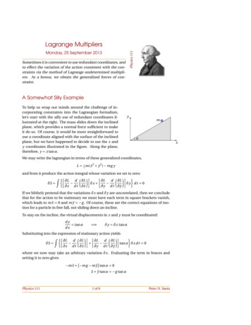
Physics 111Lagrange MultipliersMonday, 25 September 2013Sometimes it is convenient to use redundant coordinates, andto effect the variation of the action consistent with the constraints via the method of Lagrange undetermined multipliers. As a bonus, we obtain the generalized forces of constraint.A Somewhat Silly ExampleTo help us wrap our minds around the challenge of incorporating constraints into the Lagrangian formalism,let’s start with the silly use of redundant coordinates illustrated at the right. The mass slides down the inclinedplane, which provides a normal force sufficient to makeit do so. Of course, it would be more straightforward touse a coordinate aligned with the surface of the inclinedplane, but we have happened to decide to use the x andy coordinates illustrated in the figure. Along the plane,therefore, y x tan α.ymαxWe may write the lagrangian in terms of these generalized coordinates,L 12 m(ẋ 2 ẏ 2 ) mg yand from it produce the action integral whose variation we set to zero:µ ¶ ·µ ¶ ¾Z ½·d L Ld L L δx δy d t 0δS x d t ẋ y d t ẏIf we blithely pretend that the variations δx and δy are uncorrelated, then we concludethat for the action to be stationary we must have each term in square brackets vanish,which leads to m ẍ 0 and m ÿ g . Of course, these are the correct equations of motion for a particle in free fall, not sliding down an incline.To stay on the incline, the virtual displacements in x and y must be coordinated:dy tan αdx δy δx tan αSubstituting into the expression of stationary action yieldsµ ¶ ·µ ¶ ¾Z ½· Ld L Ld LδS tan α δx d t 0 x d t ẋ y d t ẏwhere we now may take an arbitrary variation δx. Evaluating the term in braces andsetting it to zero gives¡ m ẍ mg m ÿ tan α 0ẍ ÿ tan α g tan αPhysics 1111 of 6Peter N. Saeta

Differentiating the constraint equation with respect to time twice, ÿ ẍ tan α, allows usto eliminate y from the equation:ẍ ẍ tan2 α g tan αẍ sec2 α g tan αẍ g sin α cos αwhich is indeed the correct equation of motion for x.The General CaseLet’s generalize to the case of a mechanical system with N P degrees of freedom, whichwe describe with N generalized coordinates and P equations of constraint. We will assume that dissipation may be neglected so that the system may be described by a Lagrangian. Let us suppose that the equations of constraint may be written in the formG j (q i , t ) 0dG j X G ji q id qi G j tdt 0for j 1, 2, . . . , P . For notational convenience, define G j q i ajiand G j tTranslation: just to confuse you. ajtThen the j th constraint equation may be writtena j i d qi a j t d t 0ora j i q̇ i a j t 0(P equations)Note that the coefficients a j i and a j t may be functions of the generalized coordinatesq i and the time t , but not the generalized velocities q̇ i .Hamilton’s principle says that of all possible paths, the one the system follows is thatwhich minimizes the action, which is the time integral of the lagrangian:Z tbδS δL(q i , q̇ i , t ) d t 0(1)taExpanding the variation in the lagrangian and integrating by parts, we obtainµ¶ Z tb · Ld LδS δq i d t q i d t q̇ itawhich must vanish on the minimum path. When the coordinates q i formed a minimalcomplete set, we argued that the virtual displacements δq i were arbitrary and that theonly way to ensure that the action be minimum is for each term in the square bracketsto vanish.Now, however, an arbitrary variation in the coordinates will send us off the constraintsurface, leading to an impossible solution. One way to “trick” Prof. Hamilton into findingthe right solution (the solution consistent with the constraint equations) would be tosneak something inside the brackets that would make the variation in the action zeroPhysics 1112 of 6Peter N. SaetaRemember that we are using the summationconvention; we sum over i .

for displacements that take us off the surface of constraint. That’s hardly cheating; it justtakes away the incentive to cheat! If we managed to find such terms, then it wouldn’tmatter which way we varied the path; we’d get zero change in the action, to first order inthe variation. We could then treat all the variations δq i as independent.Before running that little operation, consider what it might mean for those terms to represent the generalized forces of constraint. Since the allowed virtual displacements ofthe system are all orthogonal to the constraint forces, those forces do no work and theydon’t change the value of the action integral. In fact, they are just the necessary forces toensure that the motion follows the constrained path. So, if we can figure out what termswe need to add to the lagrangian to make the illegal variations vanish, we will have alsofound the forces of constraint.Each of the constraint equations is of the form G j (q i , t ) 0, so if we were to add a multiple of each constraint equation to the lagrangian, it would leave the action unchanged.So, we form the augmented Lagrangian:L0 L λ j G j(2)where I’m using the summation convention and the λ j are Lagrange’s undeterminedmultipliers, one per equation of constraint; all may be functions of the time. Then the(augmented) action isZ t2S L0 d tt1(but since we added zero, it’s the same as the un-augmented action). By Hamilton’sprinciple, the action is minimized along the true path followed by the system. We maynow effect the variation of the action and force it to vanish: Z t2 · G j L LδS δq i δq̇ i λ jδq i d t 0 q i q̇ i q it1Integrate the middle term by parts (and remember we’re using the summation convention):µ¶ Z t2 ·d L LδS λ j a j i δq i d t 0 q i d t q̇ it1We now have N variations δq i , only N P of which are independent (since the systemhas only N P degrees of freedom). Using the P independent Lagrange multipliers, wemay ensure that all N terms inside the square bracket vanish, so that no matter what thevariations δq i the value of the integral doesn’t vary. Thus we haveµ¶d L L λj a ji(N equations)d t q̇ i q ia j i d qi a j t d t 0ora j i q̇ i a j t 0(P equations)or, if you prefer,µ¶ G jd L L λjd t q̇ i q i q i G j G j G j G jd qi dt 0orq̇ i 0 q i t q i tPhysics 1113 of 6(N equations)(P equations)Peter N. SaetaThe prime on L 0 does not imply differentiation, merely that this is the “augmented” Lagrangian function defined in Eq. (2).

Since there are N generalized coordinates and P Lagrange multipliers, we now have aclosed algebraic system.When we derived Lagrangian mechanics starting from Newton’s laws, we showed thatµ¶ T rd T Fitot Ftot ·d t q̇ i q i q iwhere F is the total force on the particle and Fitot is the generalized force correspondingto the i th generalized coordinate. If we separate the forces into those expressible interms of a scalar potential depending only on positions (not velocities), the forces ofconstraint, and anything left over, then this becomesµ¶ Ld L Ficonstraint Finoncons(3)d t q̇ i q iComparing with the N Lagrange equations above, we see that when all the forces areconservative, G j r λj a ji λjFiconstraint Fconstraint · q i q iIn other words, the sum λ j G j q iSummed over j .is the generalized constraint force.Example 1yθxA hoop of mass m and radius R rolls without slippingdown a plane inclined at angle α with respect to thehorizontal. Solve for the motion, as well as the generalized constraint forces.Using the indicated coordinate system, we have nomotion in y, but coordinated motion between x andθ, which are linked by the constraint conditionR dθ dxorR dθ dx 0αTherefore,a 1θ R,a 1x 1,2The kinetic energy is T m2 ẋ mg x sin α, so the Lagrangian isL T V mR 22a 1t 0θ̇ 2 and the potential energy is V m 2 mR 2 2ẋ θ̇ mg x sin α22We will first solve by using the constraint equation to eliminate θ: R θ̇ ẋ, soL Physics 111m 2 m 2ẋ ẋ mg x sin α m ẋ 2 mg x sin α224 of 6Peter N. Saeta

This Lagrangian has a single generalized coordinate, x, and thus we obtainthe equation of motionµ ¶ Ld Lg 0 2m ẍ mg sin α 0 ẍ sin αd t ẋ x2which is half as fast as it would accelerate if it slid without friction.If we delay the gratification of inserting the constraint and instead use thelagrangian with two generalized coordinates, we getµ ¶ Ld L λ1 a 1x m ẍ mg sin α λ1 ( 1)d t ẋ xµ ¶d L L λ1 a 1θ mR 2 θ̈ 0 λ1 Rd t θ̇ θFrom the second equation, we obtain λ1 mR θ̈ m ẍ, where I have used theconstraint equation R θ̈ ẍ in the last step. Substituting into the first equation, we again obtain ẍ g /2 sin α.What about the constraint forces? The generalized constraint force in x ismgFx λ1 a1x m ẍ 2 sin α. This is the force heading up the slope produced by friction; it is responsible for the slowed motion of the center of mass.mg RThe generalized constraint force in θ is Fθ λ1 R mR ẍ 2 sin α. This isthe torque about the center of mass of the hoop caused by the frictional force.SummaryWhen you wish to use redundant coordinates, or when you wish to determine forces ofconstraint using the Lagrangian approach, here’s the recipe:1. Write the equations of constraint, G j (q i , t ) 0, in the forma j i d qi a j t d t 0where a j i G j q i.2. Write down the N Lagrange equations,µ¶d L L λj a jid t q i q i(summation convention)where the λ j (t ) are the Lagrange undetermined multipliers and Fi λ j a j i is thegeneralized force of constraint in the q i direction.3. Solve, using the N Lagrange equations and the P constraint equations.4. Compute the generalized constraint forces, Fi , if desired.Physics 1115 of 6Peter N. Saeta

Problem 1 Use the method of Lagrange undetermined multipliers to calculate the generalized constraint forces on our venerable bead, which is forced to move without friction on a hoop of radius R whose normal is horizontal and forced to rotate at angularvelocity ω about a vertical axis through its center. Interpret these generalized forces.What do they correspond to physically?Physics 1116 of 6Peter N. Saeta

2.Write down the N Lagrange equations, d dt µ @L @q i ¶ ¡ @L @qi ‚j aji (summation convention) where the ‚j(t) are the Lagrange undetermined multipliers and Fi ‚j aji is the generalized force of constraint in the qi direction. 3.Solve, using the N Lagrange equations and the P constraint equations. 4.Compute the generalized .