WIXLIB

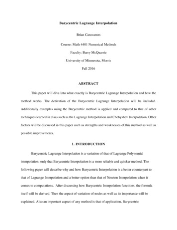
IntroductionChebyshev techniquesNumerical investigationsPolynomial interpolation toolsChebyshev interpolationChebyshev GreeksChebyshev GreeksLet f (x) be the price of a financial product as a function of theparameter x.We approximate f (m) at some point x̄ through the derivative p (m) (x̄)of the Chebyshev interpolant of f in some interval including x̄.The procedure can be be split out in the following phases:12Choose the interpolation domain H 3 x̄ and the number n ofChebyshev points.Build the Chebyshev interpolator. This amounts to:iiiiiiiv3compute Chebyshev points {xk }k 0,.,n 1 on H using an affine map;compute barycentric weights {wk }k 0,.,n 1 ;compute the differential matrices up to the desired order m;evaluate the original pricing function on the Chebyshev points toobtain the interpolation nodes {f (xk )}k 0,.,n 1 .Obtain the desired Greeks as p (m) (x̄).S. ScoleriChebyshev Greeks

IntroductionChebyshev techniquesNumerical investigationsPolynomial interpolation toolsChebyshev interpolationChebyshev GreeksAdaptive DomainsParticular attention should be paid to handle possible singularities, e.g. barriers,in the price function or its derivatives.We leverage on the following heuristics: close to a singularity, the derivatives ofthe price function show some peaks, which are higher and more localized themore the barrier date approaches in time. In this case we reduce the interpolationdomain. Away from the singularity, we can always use a wider domain.Therefore, we employ different methods to adapt the size of the interpolationdomain H : [ξ a, ξ a] (for some ξ) to the presence of a singularity at b:12time adaptivity:space adaptivity: a x̄ σ τa x̄ b where σ is the underlying ATM volatility, τ is the time to next singularity and ais the half-size of the interpolation domain, with appropriate bounds amin andamax . Moreover, if ξ x̄ we say that H is centered.If the singularity appears also in the price function, then we need to avoid that itfalls inside H: in this case, we apply a translation to H, without reducing it(uncentered space-adaptivity).S. ScoleriChebyshev Greeks

IntroductionChebyshev techniquesNumerical investigationsPolynomial interpolation toolsChebyshev interpolationChebyshev GreeksAdaptive DomainsThe above formula for time adaptivity is motivated by the following argument:assuming that singularities are generated by digital features,for digital options in Black model the scale of the singularity is given by σ τ .Graphical representation of the Chebyshev adaptive domain H(T ) in dependence onthe time to next barrier T compared to the behaviour of digital price (left panel),delta (middle panel) and gamma (right panel). Results shown for a Black digital callwith K 1, σ 0.4, r 0.S. ScoleriChebyshev Greeks

IntroductionChebyshev techniquesNumerical investigationsPolynomial interpolation toolsChebyshev interpolationChebyshev GreeksExampleIn order to assess the accuracy of Chebyshev methodology w.r.t. other techniques, weconsider a digital option in Black model and evaluate the following numerical errors:0ε (S) pn 1(S) BS (S) ,exactFD 3 pts (25 bps bump)FD 3 pts (1% bump)FD 7 ptschebyshev 7 pts17.500εΓ (S) pn 1(S) ΓBS (S)exactFD 3 pts (25 bps bump)FD 3 pts (1% bump)FD 7 ptschebyshev 7 pts8000.660025015.00.540012.50.40.37.5error (dotted lines)gammaerror (dotted lines)delta10.020020015001000.2 2002.50.1 01.07550 0751.100Method# nodesAvg ε Std ε Max ε Avg εΓStd εΓMax εΓFD 25bps bumpFD 1% bumpFD 1% bumpadaptive 0.6S. ScoleriChebyshev Greeks

IntroductionChebyshev techniquesNumerical investigations1IntroductionMotivationBias vs VarianceSmoothing2Chebyshev techniquesPolynomial interpolation toolsChebyshev interpolationChebyshev Greeks3Numerical investigationsTarget Redemption ForwardsAutocallablesWindow Barriers4ConclusionsS. ScoleriTarget Redemption ForwardsAutocallablesWindow BarriersChebyshev Greeks

IntroductionChebyshev techniquesNumerical investigationsTarget Redemption ForwardsAutocallablesWindow BarriersApplications to Real PayoffsWe now assess the effectiveness of our methodology in the computationof spot Greeks Delta and Gamma for some exotic payoffs with differenttypes of singularities:1FX Target Redemption Forwards (TARFs) under the StochasticLocal Volatility (SLV) model by [Tataru-Fisher(2010)]2Equity Autocallable options under multi-asset Local Volatility (LV)model by [Dupire(1994), Derman-Kani(1994)]We compare Chebyshev Greeks with 3-point finite difference Greeks fordifferent pricing dates and spot levels. The efficiency of the methodologycan be assessed via the average MC error, defined as1 :εt (y ) L1 XSEy (Sp )L p 11 Here,t denotes the pricing date, {Sp }p 1,.,L is a grid of spot levels (L 200 inour tests), SE denotes the standard error. Finally, y denotes price, delta or gamma.S. ScoleriChebyshev Greeks

IntroductionChebyshev techniquesNumerical investigationsTarget Redemption ForwardsAutocallablesWindow BarriersTest 1: FX TARFsWe consider a TARF KO, i.e. an FX product which pays, at each fixingdate Ti , the following put-like coupons until a maximum payout θ(target) is reached:K S Ti K S Ti1{ST K } 1{ST BKI }iiii nXo n X 1(K STj ) θ1 min 1,1{STj 1j 1In particular, we specify the following contract data:underlying asset: S EUR/USD FX ratestrike: K 1.15knock-in barrier: BKI 1.19knock-out barrier: BKO 1.135number of coupons: 70coupon frequency: weeklyresidual target: θ 0.2coupon notionals: Ni 0.3 · 1{STi K }S. Scoleri 0.6 · 1{STiChebyshev Greeks K }o j BKO }Ni

IntroductionChebyshev techniquesNumerical investigationsTarget Redemption ForwardsAutocallablesWindow BarriersTest 1: FX TARFs - Delta1 day to next fixing0 10 10 15 15 20 25 30 30 35 351.101.151.20spots1.25FD 3 ptschebyshev 20 25 40fixing date, 1 week to next fixing 5deltadelta 5 0FD 3 ptschebyshev1.301.101.151.20spots1.251.30Greeks methodMC paths# nodesaminamaxε1d ( )ε1w ( )finite differencesadaptive 040.030.03centered space-time adaptivityS. ScoleriChebyshev Greeks

IntroductionChebyshev techniquesNumerical investigationsTarget Redemption ForwardsAutocallablesWindow BarriersTest 1: FX TARFs - Gamma1 day to next fixingfixing date, 1 week to next fixingFD 3 ptschebyshev 00 200 1000 400gammagamma1000 2000 600 3000 800 4000 10001.101.151.20spots1.251.30FD 3 ptschebyshev1.101.151.20spots1.251.30Greeks methodMC paths# nodesaminamaxε1d (Γ)ε1w (Γ)finite differencesadaptive 4centered space-time adaptivityS. ScoleriChebyshev Greeks

IntroductionChebyshev techniquesNumerical investigationsTarget Redemption ForwardsAutocallablesWindow BarriersTest 2: Equity AutocallablesWe now consider an autocallable with memory on a basket of twostocks, i.e. an option paying, at each time Ti , the following coupons,unless the basket performance crosses a level Bcall : "Π(Ti ) 1{τ Ti } Ni #i 1 XNj Π(Tj ) 1{P(Ti ) Bcoup } δiN (P(TN ) 1) 1{P(TN ) Bguar } j 1where τ min{Ti : P(Ti ) Bcall }.In particular, we specify the following contract data:underlying assets: TELECOM and VODAFONE share pricesnoperformance type: “worst-of”, i.e. P(t) min StTEL /0.48, StVOD /1.3call barrier: Bcall 100%coupon barrier: Bcoup 90%capital-guarantee barrier: Bguar 60%number of coupons: N 7coupon frequency: quarterlycoupon notionals: Ni 0.02S. ScoleriChebyshev Greeks

IntroductionChebyshev techniquesNumerical investigationsTarget Redemption ForwardsAutocallablesWindow BarriersTest 2: Equity Autocallables - Delta3 days to next fixing3 months to next fixingFD 3 350 0.375 0.400 0.425 0.450 0.475 0.500 0.525spots FD 3 ptschebyshev1.6deltadelta3.00.350 0.375 0.400 0.425 0.450 0.475 0.500 0.525spotsGreeks methodMC paths# nodesaminamaxε3d ( )ε3m ( )finite differencesadaptive 01centered space-time adaptivityS. ScoleriChebyshev Greeks

IntroductionChebyshev techniquesNumerical investigationsTarget Redemption ForwardsAutocallablesWindow BarriersTest 2: Equity Autocallables - Gamma3 days to next fixing3 months to next fixingFD 3 ptschebyshev5000 5gammagamma100 50 10 15 100 20 1500.350 0.375 0.400 0.425 0.450 0.475 0.500 0.525spots FD 3 ptschebyshev0.350 0.375 0.400 0.425 0.450 0.475 0.500 0.525spotsGreeks methodMC paths# nodesaminamaxε3d (Γ)ε3m (Γ)finite differencesadaptive Chebyshev1,000,000300,000371%3%1%10%7551centered space-time adaptivityS. ScoleriChebyshev Greeks

IntroductionChebyshev techniquesNumerical investigationsTarget Redemption ForwardsAutocallablesWindow BarriersTest 3 (Beyond MC Greeks): Window UOCThe benefits of Chebyshev Greeks are not limited to MC pricers: consider e.g. anup-and-out window barrier option under the SLV model by [Tataru-Fisher(2010)],priced with a PDE approach as described in [in ’t Hout-Foulon(2010)]:Π(T ) [ω (ST K )] 1{St B, Ts t Te }We perform a similar analysis as before2 on the following contract:underlying asset: S EUR/USD FX ratecall type: ω 1strike: K 1.1574barrier level: B 1.23barrier monitoring: continuousbarrier end date Te : 11Mexpiry T : 1Y2 Regarding the estimations of errors ε (y ), we consider here the average distance,ton 200 spot levels, with values of y computed with a double-sized PDE grid and7-point FD with a bump of 5bps. The barrier start date Ts can be either future orpast, depending on the test case.S. ScoleriChebyshev Greeks

IntroductionChebyshev techniquesNumerical investigationsTarget Redemption ForwardsAutocallablesWindow BarriersTest 3 (Beyond MC Greeks): Window UOC - Delta5 days to barrier start date5 days past barrier start dateFD 3 ptschebyshev0.100.050.050.00deltadelta0.00 0.05 0.05 0.10 0.10 0.15 0.15 0.20 0.201.00 1.05 1.10 1.15 1.20 1.25 1.30spots FD 3 ptschebyshev0.101.00 1.05 1.10 1.15 1.20 1.25 1.30spotsGreeks methodx-thickness# nodesaminamaxε 5d ( )ε5d ( )finite differencesadaptive .00005centered time-adaptivity before barrier start, uncentered space-adaptivity afterwards.S. ScoleriChebyshev Greeks

IntroductionChebyshev techniquesNumerical investigationsTarget Redemption ForwardsAutocallablesWindow BarriersTest 3 (Beyond MC Greeks): Window UOC - Gamma155 days past barrier start date640 20 4 5 61.00 1.05 1.10 1.15 1.20 1.25 1.30spots FD 3 ptschebyshev25gammagamma105 days to barrier start dateFD 3 ptschebyshev1.00 1.05 1.10 1.15 1.20 1.25 1.30spotsGreeks methodx-thickness# nodesaminamaxε 5d (Γ)ε5d (Γ)finite differencesadaptive red time-adaptivity before barrier start, uncentered space-adaptivity afterwards.S. ScoleriChebyshev Greeks

IntroductionChebyshev techniquesNumerical investigations1IntroductionMotivationBias vs VarianceSmoothing2Chebyshev techniquesPolynomial interpolation toolsChebyshev interpolationChebyshev Greeks3Numerical investigationsTarget Redemption ForwardsAutocallablesWindow Barriers4ConclusionsS. ScoleriChebyshev Greeks

IntroductionChebyshev techniquesNumerical investigationsConclusions and Future PerspectivesWe presented a simple and general method, based on Chebyshevinterpolation techniques, for Greeks computation of arbitrarilycomplex payoffs, with different numerical pricing techniques.The number of interpolation nodes can be kept low (typically under10), while the size of interpolation domain can be adapted to thetime and space distance from singularities in the price or itsderivatives.In most situations, the methodology allows to significantly improvethe numerical stability of Greeks and, at the same time, to reducethe computational time, even though the number of repricings isslightly increased w.r.t. standard FD.The multi-dimensional extension3 of Chebyshev techniques wouldoffer the possibility to effectively compute also cross-gammas.3 seee.g. [Glau et al.(2020)]S. ScoleriChebyshev Greeks

IntroductionChebyshev techniquesNumerical investigationsReferencesDerman, E. and Kani, I., 1994. Riding on a smile, Risk. 7:32–39.Dupire, B., 1994. Pricing with a smile, Risk. 7(1):18–20.Glasserman, P., 2003. Monte Carlo Methods in FinancialEngineering, Springer.Gaß, M., Glau, K., Mahlstedt, M., Mair, M., 2018. Chebyshevinterpolation for parametric option pricing, Finance and Stochastics.22(3):701–731.Glau, K., Kressner, D., Statti, F., 2020. Low-rank tensorapproximation for Chebyshev interpolation in parametric optionpricing, SIAM Journal on Financial Mathematics. 11(3):897–927.in ’t Hout, K. J. and Foulon, S., 2010. ADI finite difference schemesfor option pricing in the Heston model with correlation, InternationalJournal of Numerical Analysis and Modeling, 7(2):303–320.S. ScoleriChebyshev Greeks

IntroductionChebyshev techniquesNumerical investigationsReferences (cont.)Maran, A., Pallavicini, A., and Scoleri, S., 2021. Chebyshev Greeks.Smoothing Gamma without Bias, preprint:https://ssrn.com/abstract 3872744.Tataru, G. and Fisher, T., 2010. Stochastic local volatility,Quantitative Development Group, Bloomberg.Trefethen, L.N., 2020. Approximation Theory and ApproximationPractice, SIAM – Society for Industrial and Applied Mathematics.Zeron Medina Laris, M. and Ruiz, I., 2018. Chebyshev methods forultra-efficient risk calculations, preprint:https://arxiv.org/abs/1805.00898.Zeron Medina Laris, M. and Ruiz, I., 2020. Tensoring volatilitycalibration, preprint: https://arxiv.org/abs/2012.07440.S. ScoleriChebyshev Greeks

IntroductionChebyshev techniquesNumerical investigationsReferences (cont.)Zeron Medina Laris, M. and Ruiz, I., 2021. Denting the FRTB IMAcomputational challenge via orthogonal Chebyshev sliding technique,Wilmott Magazine, 111:74–93.Zeron Medina Laris, M. and Ruiz, I., 2021. Tensoring dynamicsensitivities and dynamic initial margin, Risk, published online.DisclaimerThe opinions expressed in this work are solely those of the authors and donot represent in any way those of their current and past employers.S. ScoleriChebyshev Greeks

Finite Di erence Gamma of a digital option for di erent spot levels. Black-Scholes exact formulas are compared with MC results using 300K paths, 0.0025 bump and two di erent smoothing parameters: the smoothed Greek is biased. S. Scoleri Chebyshev Greeks. Introduction Chebyshev techniques Numerical investigations Polynomial interpolation tools Chebyshev interpolation Chebyshev Greeks 1 .