Transcription
Chapter 15. SPATIAL INTERPOLATION15.1 Elements of Spatial Interpolation15.1.1 Control Points15.1.2 Type of Spatial Interpolation15.2 Global Methods15.2.1 Trend Surface ModelsBox 15.1 A Worked Example of Trend Surface Analysis15.2.2 Regression Models15.3 Local Methods15.3.1 Thiessen Polygons15.3.2 Density EstimationBox 15.2 A Worked Example of Kernel Density Estimation15.3.3 Inverse Distance Weighted InterpolationBox 15.3 A Worked Example of Inverse Distance WeightedEstimation15.3.4 Thin-Plate SplinesBox 15.4 Radial Basis FunctionsCopyright The McGraw-Hill Companies, Inc. Permission required for reproduction or display.Box 15.5 A Worked Example of Thin-Plate Splines with Tension15.4 Kriging15.4.1 Semivariogram15.4.2 Models15.4.3 Ordinary KrigingBox 15.6 A Worked Example of Ordinary Kriging Estimation15.4.4 Universal KrigingBox 15.7 A Worked Example of Universal Kriging Estimation15.4.5 Other Kriging Methods15.5 Comparison of Spatial Interpolation MethodsBox 15.8 Spatial Interpolation Using ArcGISKey Concepts and TermsReview QuestionsApplications: Spatial InterpolationTask 1: Use Trend Surface Model for InterpolationTask 2: Use Kernel Density Estimation MethodTask 3: Use IDW for InterpolationTask 4: Use Ordinary Kriging for InterpolationTask 5: Use Universal Kriging for InterpolationChallenge QuestionReferences1
Spatial InterpolationzSpatial interpolation is the process of using points withknown values to estimate values at other points.zIn GIS applications, spatial interpolation is typically appliedto a raster with estimates made for all cells. Spatialinterpolation is therefore a means of creating surface datafrom sample points.Control PointszControl Points are points with known values. Theyprovide the data necessary for the development of aninterpolator for spatial interpolation.zThe number and distribution of control points can greatlyinfluence the accuracy of spatial interpolation.2
Figure 15.1A map of 175 weatherstations in and around Idaho.Type of Spatial Interpolation1. Spatial interpolation can be global or local.2. Spatial interpolation can be exact or inexact.3. Spatial interpolation can be deterministic or stochastic.3
Figure 15.2Exact interpolation (a) and inexact interpolation (b).Figure 15.3Estimation of the unknown value at Point 0 from fivesurrounding known points.4
chasticTrend surface(inexact)*Regression(inexact)Thiessen (exact)KrigingDensity estimation(exact)(inexact)Inverse distance weighted(exact)Splines (exact)*Given some required assumptions, trend surface analysis can be treated as a specialcase of regression analysis and thus a stochastic method (Griffith and Amrhein 1991).Table 15.1 A classification of spatial interpolation methodsGlobal MethodszTrend surface analysis, an inexact interpolation method,approximates points with known values with a polynomialequation.zA regression model relates a dependent variable to anumber of independent variables in a linear equation (aninterpolator), which can then be used for prediction orestimation.5
Figure 15.4An isohyet map from a thirdorder trend surface model.Local MethodsBecause local interpolation uses a sample of known points, itis important to know how many known points to use, and howto search for those known points.6
Figure 15.5Three search methods for sample points: (a) find the closest pointsto the point to be estimated, (b) find points within a radius, and (c)find points within each quadrant.Thiessen PolygonsThiessen polygons assume that any point within apolygon is closer to the polygon’s known point than anyother known points.7
Figure 15.6Thiessen polygons (in thicker lines) are interpolated from theknown points and the Delaunay triangulation (in thinner lines).Density EstimationzDensity estimation measures cell densities in a raster byusing a sample of known points.zThere are simple and kernel density estimation methods.8
Figure 15.7Deer sightings per hectare calculated by the simple density estimation method.Figure 15.8A kernel function, which represents a probability densityfunction, looks like a “bump” above a grid.9
Figure 15.9Deer sightings perhectare calculated bythe kernel estimationmethod. The letter Xmarks the cell, which isused as an example inBox 15.2.Inverse Distance WeightedInterpolationInverse distance weighted (IDW) interpolation is an exactmethod that enforces that the estimated value of a point isinfluenced more by nearby known points than those fartheraway.10
Figure 15.10An annual precipitationsurface created by theinverse distancesquared method.Figure 15.11An isohyet map createdby the inverse distancesquared method.11
Thin-Plate SplinesThin-plate splines create a surface that passes throughthe control points and has the least possible change inslope at all points. In other words, thin-plate splines fitthe control points with a minimum curvature surface.Figure 15.12An isohyet map createdby the regularizedsplines method.12
Figure 15.13An isohyet map createdby the splines withtension method.KrigingzKriging is a geostatistical method for spatial interpolation. Kriging canassess the quality of prediction with estimated prediction errors.zKriging assumes that the spatial variation of an attribute is neithertotally random (stochastic) nor deterministic. Instead, the spatialvariation may consist of three components: a spatially correlatedcomponent, representing the variation of the regionalized variable; a“drift” or structure, representing a trend; and a random error term.zThe interpretation of these components has led to development ofdifferent kriging methods for spatial interpolation.13
SemivariogramzKriging uses the semivariance to measure the spatially correlatedcomponent, a component that is also called spatial dependence orspatial autocorrelation.zA semivariogram cloud plots semivariance against distance for allpairs of known points in a data set. If spatial dependence does existin a data set, known points that are close to each other areexpected to have small semivariances and known points that arefarther apart are expected to have larger semivariances.Figure 15.14A semivariogram cloud.14
BinningWith all pairs of known points, a semivariogram cloud isdifficult to manage and use. Binning is a process thataverages semivariance data by distance and direction.Figure 15.15A common method for binning pairs of sample points by direction,such as 1 and 2 in (a), is to use the radial sector (b). GeostatisticalAnalyst to ArcGIS uses grid cells instead (c).15
Figure 15.16A semivariogram after binning by distance.Model FittingA semivariogram must be fitted with a mathematical functionor model so that it can be used for estimating thesemivariance at any given distance.16
Figure 15.17Fitting a semivariogram with a mathematical function or a model.Figure 15.18Two common models for fitting semivariograms: spherical and exponential.17
Nugget, Range, and SillzThe nugget is the semivariance at the distance of 0,representing measurement error, or microscale variation,or both.zThe range is the distance at which the semivariancestarts to level off.zThe sill is the semivariance at which the leveling takesplace.Figure 15.19Nugget, range, sill, and partial sill.18
Ordinary KrigingAssuming the absence of a drift, ordinary kriging focuses onthe spatially correlated component and uses the fittedsemivariogram directly for interpolation.Figure 15.20An isohyet map createdby ordinary kriging withthe exponential model.19
Figure 15.21Standard errors of theannual precipitationsurface in Figure 15.20.Universal KrigingUniversal kriging assumes that the spatial variation in z valueshas a drift or a trend in addition to the spatial correlationbetween the sample points.20
Figure 15.22An isohyet mapcreated by universalkriging with the lineardrift and the sphericalmodel.Figure 15.23Standard errors ofthe annualprecipitation surfacein Figure 15.22.21
Comparison of Spatial InterpolationMethodsUsing the same data but different methods, we can expect to finddifferent interpolation results. Likewise, different predicted values canoccur by using the same method but different parameter values.Figure 15.24Differences between theinterpolated surfaces fromordinary kriging and IDW.22
3
Spatial Interpolation zSpatial interpolation is the process of using points with known values to estimate values at other points. zIn GIS applications, spatial interpolation is typically applied . Analyst to ArcGIS uses grid cells instead (c). 16 Figure 15.16 A semivariogram after binning by distance. Model Fitting