Transcription
Subsea Open Cables: A Practical Perspective onthe Guidelines and GotchasSubmitted to SubOptic 2019 on April 7, 2019SubOptic Open Cables Working Group Contributors & White Paper Authors:Elizabeth Rivera Hartling, Facebook (Editor)Pascal Pecci, ASNPriyanth Mehta, CienaDarwin Evans, CienaValey Kamalov, GoogleMattia Cantono, GoogleEduardo Mateo, NECFatih Yaman, NECAlexei Pilipetskii, SubcomChris Mott, TelstraPaul Lomas, TelstraPhilip Murphy, TelstraA Brief Introduction to the Working Group, our Mission, and the Intent of this White Paper:This white paper is a collaborative work, written and discussed by the authors and contributors listed.It is intended as a means to share with the broader industry some collectively agreed ideas andrecommendations on Open Cables, from a broad representation of industry experts with varyingperspectives and practical experience in designing and building Open Cables. It attempts to lay afoundation upon which standardization via official standards bodies can build on and progress.It is by no means comprehensive, nor set in stone, as the topics covered are highly nuanced, and theindustry and core technologies are constantly evolving, and will no doubt continue to do so. It insteadattempts to provide a practical perspective on some key technical topics, as agreed and understood tothe best of our knowledge today, that will empower new entrants to the Subsea Open Cable movementto confidently embrace the ideas and reap the benefits made available by doing so.
Table of ContentsSubsea Open Cables: A Practical Perspective on the Guidelines and Gotchas . 1Why Open Cables? A Brief History . 3The Road to Open Cables .3Discussing the Benefits of Open Cables.3Open Cables Giving Rise to New Challenges .4Introduction of OSNR and GSNR as Paired Metrics . 8OSNR Definitions and Conversion into SNRASE .8GOSNR Definitions and Conversion into GSNR . 10Measuring our Defined Metrics . 12SNRASE and GSNR Measurement Introduction . 12GSNR Measurement Principle. 13GSNR Measurement Procedure. 15Discussing the Impact of Errors . 22The Relative Impact of SNRASE and SNRNLI on GSNR . 22The Impact of SNRMODEM and GSNR on Capacity Estimation . 23Modem Capacity Quantization and the Impact on Risk . 30Considering the Architecture of Open Cables . 33ITU Standardization Work . 33Coupling Considerations . 34Supervisory Considerations . 35What to Ask for in an Open Cable ITT . 37Why Traditional Capacity-based ITTs are no Longer Sufficient . 37How Open Cables Can Overcome the Traditional ITT Limitations . 39Setting Capacity Targets and Assessing Individual Risk Tolerance . 39Setting Wet Plant Optical Performance Design Targets . 41Specifying, Commissioning & Accepting an Open Cable. 44Data Differences Before & After RFS . 44Design Specifications & Acceptance Criteria . 44Commissioning & Acceptance Testing. 48Spectrum Sharing. How does GSNR vs Frequency Help?. 53The Old Adage: Not All Spectrum is Created Equal . 53Strategies for Sharing Spectrum Equitably . 53Spectrum Sharing and Trending Towards SDM. 55References . 56
Why Open Cables? A Brief HistoryThe Road to Open CablesHistorically, the definition and characterization of transmission performance for optical subsea links hasbeen based on power budget tables where the metric for channel performance was the Q-factor asprescribed by ITU-T standards G-976 and G-977 [1,2,3]. This approach was originally derived for intensitymodulation formats with direct detection (IMDD) systems, as the Q-factor could be directly related to theeye diagram of the received signal [1]. In this context, the total transmission capacity of an optical cablewas estimated using a simplified performance budget accounting for factors such as the linear noiseaccumulation, the channel spacing, total system operating bandwidth and various other calculated orsimulated penalties. Such a simplified approach was acceptable as systems were designed end-to-end,optimizing the wetplant (i.e. its dispersion maps) for the specific SLTE to be deployed. This unified end-toend design was an ideal approach at the time, under the assumption that the wetplant and SLTE wouldbe provided by the same supplier over the system lifetime. [4]The advent of transponders based on polarization multiplexed, multilevel modulation formats with DSPenabled coherent receivers completely changed the industry approach to coupling of wetplant and SLTE.DSP-enabled coherent transponders offered unprecedented flexibility in SLTE operations, offeringelectronic chromatic dispersion (CD) and polarization mode dispersion (PMD) compensation, and puttingmany different modulation formats, symbol rates, FEC and thus line rates within a single box. At itsinception, the market availability and performance of coherent transponders for use on dispersionmanaged wetplant were widely varying and offered significant capacity improvements over the IMDDtransponders originally designed for. As such, it was often highly beneficial to replace the originallyinstalled SLTE, leading to the emergence of the “upgrade market”, and the first step toward wetplant andSLTE disaggregation in the industry, or “Open Cables”. [4]An arguably more significant side effect of these new coherent transponders in the path towards OpenCables, with the newly offered ability to digitally compensate CD, was the enablement of significant wetplant design simplification via removal of inline dispersion management [13,14]. This wetplant design shiftlaid the foundation for new modem-independent performance metrics, by significant simplification of themodeling of fiber propagation impairments, and the ability to reasonably de-couple the wetplant andtransponder noise contributions.Discussing the Benefits of Open CablesThe benefits of Open Cables have been touted extensively in the industry. One often highlighted benefitis the enablement of independent vendor selection for wet plant and SLTE, allowing best of breedutilization on two very critical pieces of the subsea network. [6,7]
Figure 1. An Open Subsea Cable.Since SLTE technology cycles are typically faster than a Submarine cable build cycle, and chipgenerations are inherently staggered in timing across multiple DSP vendors, this independent selectionallows absolute maximization of cable capacity at the time of cable RFS.Just as critically, Open Cables enable the use of preferred SLTE vendors, which is essential operationallywhen considering a global subsea & terrestrial mesh network. Yet this model still supports wet plantselection from any vendor, something not as easily done in the traditional turnkey models. As such, OpenSubsea Cables enable Open Networks on a global scale.Figure 2. Open Cables to Open Networks.Open Cables Giving Rise to New ChallengesThe Open Cable model also presents a new challenge, where now a means to quantify the wetplantperformance independently of a specific SLTE or modem technology is needed. A traditional turnkeycapacity specification is no longer of great use, as it is firmly tied to one specific modem vendortechnology and indicates very little about the relative performance potential of different wetplantdesigns offered by different vendors, making comparison during an ITT process difficult.Capacity potential of a specific wetplant design must also now be viewed as a moving target, in that it isvariable in time due to its inherent tie to SLTE vendor technology and their associated generationalrelease dates. Thus, the capacity that can be delivered by a particular wet plant design, is both highlydependent on the SLTE technology choice and the time at which the cable goes RFS.
Furthermore, beyond cable RFS, the ongoing monitoring of the performance and effects of aging andmaintenance on any subsea cable throughout its operational lifetime is also of great importance.Monitoring the health and performance of a subsea cable with a single SLTE and its associatedperformance metrics may be very useful while that SLTE technology is deployed, but that data is noteasily carried over nor related to the unique performance metrics of the next generation of SLTEtechnology that may replace it.This leads to the logical conclusion that one or more performance metrics are needed that areimmutable with respect to SLTE technology and time.It has been proposed within the industry that OSNR and GSNR are the key metrics that can be used tocomprehensively describe the optical performance of a particular wetplant design, assuming a modernday D fiber design [4]. It is important to note that this proposal suggests that both OSNR and GSNR arerequired, together, to fully describe the optical performance, and that neither metric in isolation willprovide a complete picture. More details on OSNR and GSNR are provided in the sections that follow,beginning with their definitions in “Introduction of OSNR and GSNR as Paired Metrics”.OSNR has many good attributes as a performance metric – it is well understood and straightforward tocalculate, define and measure in a repeatable way by any vendor. It is also the primary contributor tothe overall optical performance levels (i.e. noise) in modern day D subsea designs, particularly as SDMdesign strategies become more prevalent. However, it is very important to understand that the sameOSNR can be achieved with many different wet plant designs, all with varying degrees of nonlinearity,resulting in differing capacity potentials at a given point in time with a given SLTE technology (notingthat this variance decreases in SDM designs). These variances and the relative contributions of linearand nonlinear noise are discussed in more detail in this document in “
Discussing the Impact of Errors ”.Similarly, GSNR is also not all-telling in isolation, as it does not capture potential benefits from SLTEtechnologies with nonlinear mitigation or compensation techniques. For example, two wetplant designswith the same GSNR will not necessarily give the same capacity potential, even with the same modem. Ifone wetplant design has the same GSNR, but a higher OSNR, one can deduce that design has highernonlinearity, which may, perhaps counterintuitively, present opportunity for higher performance gainsfrom a modem with appropriately matched nonlinear compensation techniques.The key conclusion is thus that the combination of both OSNR and GSNR is required for a comprehensiveunderstanding of optical performance on a D design, enabling accurate and comparable 3rd party SLTEcapacity estimates. A fictitious example of three optical designs and the various ways to compare themis provided below to illustrate these nuances.Comparing on Design Capacity only:Vendor B appears as the clear leaderWetplant DesignTurnkey-Style Design CapacityWetplant OSNRWetplant GOSNRShannon Capacity(OSNR-based)3rd Party SLTE Capacity(Based on OSNR & GOSNR)Vendor A15 Tb/s17 dB14 dBVendor B18 Tb/s17 dB15 dBVendor C16 Tb/s18 dB15 dB37.3 Tb/s37.3 Tb/s40.2 Tb/s18 Tb/s19 Tb/s20 Tb/s*Capacity, OSNR and GOSNR values are completely fictitious and for example only!Comparing on OSNR only:Perhaps Vendor C is the best?Comparing on GOSNR only:Vendors B & C appear equal?Comparing Shannon Capacity only:As Shannon is tied only to linearOSNR, this gives the same result ascomparing on OSNR only.Comparing 3rd party SLTE Capacity(at a specific reference point in time):Vendor C wet design provides mostcapacity potential when consideringBOTH OSNR and GOSNR!Figure 3. Comparing Wetplant Designs.Key Takeaways: Open Cables have many benefits, including capacity maximization at system RFS, and allowingindependent best of breed selection for both wetplant and SLTE technologiesNew wetplant performance metrics are required that are fully independent from SLTEo Comparing wetplant designs based on traditional turnkey capacity can be highlymisleadingo Ongoing monitoring of wetplant performance over the system lifetime must havecontinuity and meaning regardless of SLTE technology usedOSNR and GSNR, when considered together, can give a clear picture of the optical performanceof a subsea system, offer a fair comparison between different wetplant designs, and enable 3rdparty SLTE capacity estimation
Introduction of OSNR and GSNR as Paired MetricsIn order to properly discuss the nuances of OSNR and GSNR in relation to designing an Open Cable, wemust first define each metric with consistency and clarity. This section will introduce the definitions, thevariations that exist and what is included or excluded for each, such that the language used to describethese important concepts is well understood.OSNR Definitions and Conversion into SNRASEIn subsea optical transmission, OSNR is the Optical Signal to Noise Ratio, describing the relative noiseintroduced by the repeaters along the subsea line, as a result of Amplified Spontaneous Emission (ASE),also known as OSNRASE. However, OSNR is not an absolute value, and is highly dependent on theconditions under which it is defined. There are a number of OSNR values that are often used in OpenCable designs, such as Design OSNR, Nominal OSNR and Commissioning OSNR.It is important to note that OSNR, when defined in its most commonly used units of dB/0.1nm, is highlydependent on the reference channel count, or more accurately, the signal power contained within thedefined channel width. For simplification, it is common (for historical reasons) to use 120 channels as areference, however any channel count could be used, as long as it is consistently used. In fact, definingOSNR as a pure ratio in units of dB, also known as SNR (or SNRASE), eliminates this potential area ofconfusion when dealing with variable baud rates and channel counts, and is discussed later in thissection.OSNR is also variable with frequency across the available optical bandwidth. As such, using OSNR as anaverage value is helpful in simplifying discussions. A Worst Case OSNR, or the lower bound, of all thechannels can also be defined.The Design OSNR (average) is calculated using the classical formula:OSNRDesign 58 PTOP-NCh-G-NF-NR (average, per channel, in dB/0.1nm)where:58 is a constant related to the central wavelength of the spectrumPTOP is the EDFA output power within the repeater in dBmNCh is the number of channels in dBG is repeater gain in dBNF is the noise figure of the repeater in dBNR is the number of repeaters in dBThe Design OSNR has the advantage to be very simple to calculate based on high level systemspecifications but does not take into account all the impairments that will be present in a practicalsystem. As such, a second OSNR value is often quoted, called the Nominal OSNR (average). This OSNR isbased on the Design OSNR, beyond which any path ROADM penalties are added, and the droop isconsidered.OSNRNominal OSNRDesign-ROADM Penalties-DroopASE (average in dB)
Under ideal conditions, OSNRNominal should represent a field measurable quantity. However, due to realworld non-idealities and variations, some additional margins are generally considered. These marginsaccount for effects such as variations in fiber loss from expectations, or variability in repeater TOP fromnominal, as examples. As a consequence, a Commissioning OSNR is defined. System acceptance is thendefined around the specified Commissioning OSNRs, typically considering average and worst case.OSNRCommissioning OSNRNominal-Manufacturing Margins (average in dB)OSNR120ch (dB/0,1nm)Finally, the Worst Case Commissioning OSNR is also defined. During commissioning and acceptance,each channel individually should be above this Worst Case OSNRCommissioning.Average OSNRDesignROADM Penalties, ASE Droop.Average OSNRNominalManufacturing MarginsAverage OSNRCommissioningFrom Average to WorstWorst OSNRCommissioningFigure 4. OSNR Definitions.As previously discussed, defining OSNR with respect to 120 channels is somewhat arbitrary andhistorically based, due to the advent of Open Cables at a time when 37.5GHz channel spacing and 4.5THz repeater bandwidths were most common (allowing 120 channels). With the advent of variable baudrate transponders, a more logical reference may be to define OSNR (dB/0.1nm) as SNRASE (dB), removingany dependency on a specific channel count or spacing. OSNR can be very simply converted into SNRASEby using the following conversion:SNRASE (dB) OSNR(dB/0.1nm) – 10*LOG10(SignalBandwidth GHz / 12.5 GHz)Here, the reference bandwidth is equal to 12.5GHz since the OSNR is usually given for 0.1nm, or12.5GHz at 1550nm, and the Signal Bandwidth is the spectral width within which the channel undertest is defined. If we take a 37.5 GHz spacing, which is a classical spacing for a 30-35GBd transponder,the SNRASE will be 10*LOG10(37.5/12.5) or 4.8dB lower than the OSNR.There is an additional benefit to using SNR, as defined here within the full signal bandwidth, from atransmission performance assessment perspective, as it more accurately represents the noise that acoherent receiver will be presented with. [17] In this case, the relationship between baud rate andchannel spacing must also be accounted for.The previous set of key OSNR values could then be re-cast in a baud rate and channel spacingindependent SNR-based manner, as below.
SNRASE (dB)Average SNRDesignROADM Penalties, ASE Droop.Average SNRNominalManufacturing MarginsAverage SNRCommissioningFrom Average to WorstWorst SNRCommissioningFigure 5. SNRASE Definitions.GOSNR Definitions and Conversion into GSNRAs discussed previously, Open Cable systems requires a performance metric for assessing the opticalperformance of the wetplant which is as independent as possible of the SLTE modem. It is prudent torecall that the contents of this section are specifically defined within the bounds of a modern day D wetplant design application space.In dispersion uncompensated transmission scenarios, it has been extensively shown that fiberpropagation impairments caused by the interplay of loss, chromatic dispersion and Kerr nonlinearity canbe approximated as an additive white Gaussian noise (AWGN) or disturbance on any single frequency,named nonlinear interference (NLI)[1,2]. As all major propagation impairments, i.e. ASE and NLI, can bemodeled as Gaussian disturbances, a unique metric in the form of a signal-to-noise ratio (SNR) can beused to assess the optical performance potential of a particular defined channel within a specificwetplant design. This metric has been defined as effective or Generalized OSNR (GOSNR).Per the previous section, it is desirable to define these metrics in a channel width and baud rateindependent fashion, and as such Generalized SNR (GSNR) is introduced and defined as the ratiobetween the power of useful signal, divided by the sum of the powers of all noise sources - such as ASEand NLI - evaluated wholly in the signal bandwidth.GSNR is thus defined (in linear units) as: [4]111 𝐺𝑆𝑁𝑅 𝑆𝑁𝑅𝐴𝑆𝐸 𝑆𝑁𝑅𝑁𝐿𝐼where:- SNRASE is the channel width independent OSNR previously defined- SNRNLI is the noise coming from the nonlinear interferenceNote, for simplicity, we are focusing in the effects of fiber nonlinearity in the characterization of opensubmarine cables. However, other propagation impairments can be included in this formalism. In
particular, GAWBS, which can be well modelled in SNR terms and it depends of the fiber type andtransmission distance. As discussed in the previous section, calculating SNRASE is relativelystraightforward. Modeling SNRNLI, on the other hand, is more complex and relies on time consumingnumerical simulations or approximated analytical models. Analytical models are often favored for theirlimited numerical complexity that allows quick estimations of propagation impairments. One of themost used analytical models to achieve this, is the Gaussian Noise (GN) model [1]. Additional details onthe conditions required to utilize this model, and the relative accuracy can be found in [4], within whichit is recommended that the GN model be used in order to model the SNRNLI in subsea optical links,specifically ([10], Eq. 11).Like OSNR, GSNR carries with it the same variability with frequency in an optical spectrum, and thus istypically defined as an average value, bounded upward by a worst case value. GSNR will also beimpacted by additional real-world manufacturing variances that cannot be fully predicted by advancesimulation, such as repeater tilt and gain deviations during manufacturing and system deployment,introducing additional nonlinear noise contributions, and thus impacting the GSNR that may bemeasured at system commissioning.GSNR (dB)Logically the, like OSNR, a range of GOSNR values are also defined: Theoretical GSNR, CommissioningGSNR, Worst Case GSNR. During commissioning and acceptance, the average value of measuredchannels should be above the GSNRCommissioning (average), and each channel individually should be abovethe Worst Case GSNRCommissioning. More discussion and proposed guidelines for Commissioning &Acceptance of Open Cables is given later in this document.Average GSNRCommissioningFrom Average to WorstWorst GSNRCommissioningFigure 6. GSNR Definitions.Key Takeaways: It is desirable, with the prevalence of variable baud rate modem technologies, to define OSNRand GOSNR (as they are most commonly known) in a baud rate and channel spacingindependent manner, giving rise to their replacement by SNRASE and GSNR, respectively. GSNR represents the total sum of all linear (SNRASE) and nonlinear (SNRNLI) noise in a given opticaldesign, and is valid only in modern D cable designs (dispersion uncompensated) A range of SNRASE and GSNR values should be defined to reflect both the theoretical calculationsand practical considerations of a subsea system, such as Design SNRs, Average CommissioningSNRs, and Worst Case Commissioning SNRs.
Measuring our Defined MetricsSNRASE and GSNR Measurement IntroductionA performance metric is only as useful and accurate as its practical measurement allows it to be. Thissection will explain the methodology to measure the GSNR of a fiber-optic line, as per the definitionsprovided in the previous section.As a reminder, GSNR is a signal to noise ratio magnitude where the noise includes ASE from amplifiersand Noise from fiber nonlinearities, such as SPM, XPM and FWM. This formalism is valid as long as thesenoises can be regarded as Gaussian distributed. This is the case in modern fiber-optic transmission linedesigns, due to the large pulse spreading induced by large chromatic dispersion and represents thetarget application space for this discussion.SNRASE can be obtained using well calibrated Optical Spectrum Analyzers (OSAs) that accurately measurethe optical power in a given bandwidth. The typical procedure for measurement is well understood withgenerally accepted accuracy, when performed properly, to be within roughly 0.1 dB in error.It is important to note, however, that ASE noise level is not independent from the transmitted WDMsignal. It is a function of the amplifier operating point, which in turn depends on the spectral loadinginjected at the input of the amplifier. As such, loading conditions should be carefully selected andcontrolled to align with the desired conditions for characterization. It is recommended that theseconditions align with the most likely conditions under which the transponder of choice will be deployed.Most notably, for accurate GSNR measurement, it is critical that the spectral loading and pre-emphasisconditions chosen are identical for both the SNRASE and SNRNLI measurements, in order for the combinedresult to be meaningful [4].The value of SNRNLI is related to the power of the nonlinear products generated in a given referencebandwidth and is not straightforward to measure directly. However, it is possible to indirectly measureits effect with a well characterized digital coherent transponder, but this method requires carefulconsideration and de-coupling of impairments introduced by the measurement tool. For example,propagation associated penalties such as CD, PMD and PDL penalties will be associated with the testinstrument (coherent modem) and will vary depending on the modem technology or vendor used.As such, we define a new parameter, SNRTOT, that captures these additional penalties. SNRTOT, likeSNRASE, is a directly measurable parameter.SNRTOT is thus defined (in linear units) as:1111 𝑆𝑁𝑅𝑇𝑂𝑇 𝑆𝑁𝑅𝐴𝑆𝐸 𝑆𝑁𝑅𝑁𝐿𝐼 𝑆𝑁𝑅𝑀𝑂𝐷𝐸𝑀Or:111 𝑆𝑁𝑅𝑇𝑂𝑇 𝐺𝑆𝑁𝑅 𝑆𝑁𝑅𝑀𝑂𝐷𝐸𝑀
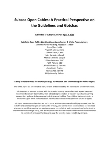
where:- GSNR, SNRASE and SNRNLI are as previously defined- SNRMODEM is the additional noise arising from the specific modem technology usedQ-factorIn this paper, the method suggested to determine the GSNR is the Inverse Back-to-Back (BtoB-1) method[8,9,11], which is based on the dependency of a transponder BER (Q-value) on fiber nonlinearities thatcreate a Gaussian-like distribution of the constellation points in the IQ space. A conceptual diagram ofthe method is provided below and will be discussed in more detail in the coming text.After transmissionBack-to-backDSNRMODEMSNRTOT GSNRSNRSNRASESNRFigure 7. GSNR measurement concept using a coherent modem.Recently, some alternate methods have been proposed based either on evaluation of spectralbroadening of a channel after transmission [16] or measuring some noise correlations on within thechannel bandwidth [15]. It is not yet clear whether proposed methods can achieve sufficient accuracy.This leaves us with the indirect measurement method using coherent transponder performance, as thebest option at this time.GSNR Measurement PrincipleIn this section, a method is introduced to measure the GSNR of a transmission line. This procedure isbased on two fundamental ideas or conditions:1- The transmission line can be well modeled by the Gaussian noise model2- Digital coherent transponders show a predictable dependency of BER with fiber nonlinearityIf these two conditions are met, the BtoB-1 method is used to estimate the GSNR of a transmission line.This method converts the Q-value of a transponder after transmission into SNRASE (or OSNR) terms, byusing the back-to-back SNRASE sensitivity of the transponder as the conversion function.The first step to
Subsea Cables enable Open Networks on a global scale. Figure 2. Open Cables to Open Networks. Open Cables Giving Rise to New Challenges The Open Cable model also presents a new challenge, where now a means to quantify the wetplant performance independently of a specific SLTE or modem technology is needed. A traditional turnkey