Transcription
Data MiningPractical Machine Learning Tools and TechniquesSlides for Chapter 7 of Data Mining by I. H. Witten and E. Frank
Engineering the input and output Attribute selection Attribute discretization Data cleansing, robust regression, anomaly detectionMeta learning Principal component analysis, random projections, text, time seriesDirty data Unsupervised, supervised, error vs entropy based, converse of discretizationData transformations Scheme independent, scheme specificBagging (with costs), randomization, boosting, additive (logistic) regression,option trees, logistic model trees, stacking, ECOCsUsing unlabeled data Clustering for classification, co training, EM and co trainingData Mining: Practical Machine Learning Tools and Techniques (Chapter 7)2
Just apply a learner? NO! Scheme/parameter selectiontreat selection process as part of the learningprocess Modifying the input: Data engineering to make learning possible oreasierModifying the output Combining models to improve performanceData Mining: Practical Machine Learning Tools and Techniques (Chapter 7)3
Attribute selection Adding a random (i.e. irrelevant) attribute cansignificantly degrade C4.5’s performance IBL very susceptible to irrelevant attributes Problem: attribute selection based on smaller andsmaller amounts of dataNumber of training instances required increasesexponentially with number of irrelevant attributesNaïve Bayes doesn’t have this problemRelevant attributes can also be harmfulData Mining: Practical Machine Learning Tools and Techniques (Chapter 7)4
Scheme independent attribute selection Filter approach: assess based on general characteristics of the dataOne method: find smallest subset of attributes that separates dataAnother method: use different learning scheme IBL based attribute weighting techniques: e.g. use attributes selected by C4.5 and 1R, or coefficients of linearmodel, possibly applied recursively (recursive feature elimination)can’t find redundant attributes (but fix has been suggested)Correlation based Feature Selection (CFS): correlation between attributes measured by symmetric uncertainty:H B H A , B U A ,B 2 H A [0,1]H A H B goodness of subset of attributes measured by (breaking ties in favor ofsmaller subsets): j U A j , C / i j U A i , A j Data Mining: Practical Machine Learning Tools and Techniques (Chapter 7)5
Attribute subsets for weather dataData Mining: Practical Machine Learning Tools and Techniques (Chapter 7)6
Searching attribute space Number of attribute subsets isexponential in number of attributesCommon greedy approaches: forward selectionbackward eliminationMore sophisticated strategies: Bidirectional searchBest first search: can find optimum solutionBeam search: approximation to best first searchGenetic algorithmsData Mining: Practical Machine Learning Tools and Techniques (Chapter 7)7
Scheme specific selection Wrapper approach to attribute selectionImplement “wrapper” around learning scheme Time consuming greedy approach, k attributes k2 time prior ranking of attributes linear in kCan use significance test to stop cross validation forsubset early if it is unlikely to “win” (race search) Evaluation criterion: cross validation performancecan be used with forward, backward selection, prior ranking, or special purpose schemata searchLearning decision tables: scheme specific attributeselection essentialEfficient for decision tables and Naïve BayesData Mining: Practical Machine Learning Tools and Techniques (Chapter 7)8
Attribute discretization Avoids normality assumption in Naïve Bayes andclustering1R: uses simple discretization schemeC4.5 performs local discretizationGlobal discretization can be advantageous becauseit’s based on more dataApply learner to k valued discretized attribute or tok – 1 binary attributes that code the cut pointsData Mining: Practical Machine Learning Tools and Techniques (Chapter 7)9
Discretization: unsupervised Determine intervals without knowing class labels Two strategies: When clustering, the only possible way!Equal interval binningEqual frequency binning(also called histogram equalization)Normally inferior to supervised schemes inclassification tasks But equal frequency binning works well with naïve Bayes ifnumber of intervals is set to square root of size of dataset(proportional k interval discretization)Data Mining: Practical Machine Learning Tools and Techniques (Chapter 7)10
Discretization: supervised Entropy based methodBuild a decision tree with pre pruning on theattribute being discretized Use entropy as splitting criterionUse minimum description length principle as stoppingcriterionWorks well: the state of the artTo apply min description length principle: The “theory” is the splitting point (log2[N – 1] bits) plus class distribution in each subsetCompare description lengths before/after adding splitData Mining: Practical Machine Learning Tools and Techniques (Chapter 7)11
Example: temperature attributeTemper at ur e6465686970717272757580818385Pl ayYesNoYes Yes YesNoNoYes Yes YesNoYes YesNoData Mining: Practical Machine Learning Tools and Techniques (Chapter 7)12
Formula for MDLP N instances Original set:k classes, entropy EFirst subset:k1 classes, entropy E1Second subset:k2 classes, entropy E2gain log2 N 1 N log2 3k 2 kE k 1 E1 k2 E2NResults in no discretization intervals fortemperature attributeData Mining: Practical Machine Learning Tools and Techniques (Chapter 7)13
Supervised discretization: other methods Can replace top down procedure by bottom upmethodCan replace MDLP by chi squared testCan use dynamic programming to find optimumk way split for given additive criterion Requires time quadratic in the number of instancesBut can be done in linear time if error rate is usedinstead of entropyData Mining: Practical Machine Learning Tools and Techniques (Chapter 7)14
Error based vs. entropy based Question:could the best discretization ever have twoadjacent intervals with the same class?Wrong answer: No. For if so, Collapse the twoFree up an intervalUse it somewhere else(This is what error based discretization will do)Right answer: Surprisingly, yes. (and entropy based discretization can do it)Data Mining: Practical Machine Learning Tools and Techniques (Chapter 7)15
Error based vs. entropy basedA 2 class,2 attributeproblemEntropy based discretization can detect change of class distributionData Mining: Practical Machine Learning Tools and Techniques (Chapter 7)16
The converse of discretizationMake nominal values into “numeric” ones1. Indicator attributes (used by IB1) Makes no use of potential ordering information2. Code an ordered nominal attribute into binaryones (used by M5’) Can be used for any ordered attributeBetter than coding ordering into an integer (whichimplies a metric)In general: code subset of attribute values asbinaryData Mining: Practical Machine Learning Tools and Techniques (Chapter 7)17
Data transformations Simple transformations can often make a large differencein performanceExample transformations (not necessarily forperformance improvement): Difference of two date attributesRatio of two numeric (ratio scale) attributesConcatenating the values of nominal attributesEncoding cluster membershipAdding noise to dataRemoving data randomly or selectivelyObfuscating the dataData Mining: Practical Machine Learning Tools and Techniques (Chapter 7)18
Principal component analysis Method for identifying the important “directions”in the dataCan rotate data into (reduced) coordinate systemthat is given by those directionsAlgorithm:1. Find direction (axis) of greatest variance2. Find direction of greatest variance that is perpendicularto previous direction and repeat Implementation: find eigenvectors of covariancematrix by diagonalization Eigenvectors (sorted by eigenvalues) are the directionsData Mining: Practical Machine Learning Tools and Techniques (Chapter 7)19
Example: 10 dimensional data Can transform data into space given by components Data is normally standardized for PCA Could also apply this recursively in tree learnerData Mining: Practical Machine Learning Tools and Techniques (Chapter 7)20
Random projections PCA is nice but expensive: cubic in number ofattributesAlternative: use random directions(projections) instead of principle componentsSurprising: random projections preservedistance relationships quite well (on average) Can use them to apply kD trees to high dimensional dataCan improve stability by using ensemble ofmodels based on different projectionsData Mining: Practical Machine Learning Tools and Techniques (Chapter 7)21
Text to attribute vectors Many data mining applications involve textual data (eg. stringattributes in ARFF)Standard transformation: convert string into bag of words bytokenization Attribute values are binary, word frequencies (f ),ijlog(1 fij), or TF IDF:f ij log ## documentsdocuments that include word i Only retain alphabetic sequences? What should be used as delimiters? Should words be converted to lowercase? Should stopwords be ignored? Should hapax legomena be included? Or even just the k mostfrequent words?Data Mining: Practical Machine Learning Tools and Techniques (Chapter 7)22
Time series In time series data, each instance represents a differenttime stepSome simple transformations: Shift values from the past/future Compute difference (delta) between instances (ie.“derivative”)In some datasets, samples are not regular but time isgiven by timestamp attribute Need to normalize by step size when transformingTransformations need to be adapted if attributesrepresent different time stepsData Mining: Practical Machine Learning Tools and Techniques (Chapter 7)23
Automatic data cleansing To improve a decision tree: Better (of course!): Remove misclassified instances, then re learn!Human expert checks misclassified instancesAttribute noise vs class noise Attribute noise should be left in training set(don’t train on clean set and test on dirty one)Systematic class noise (e.g. one class substituted foranother): leave in training setUnsystematic class noise: eliminate from trainingset, if possibleData Mining: Practical Machine Learning Tools and Techniques (Chapter 7)24
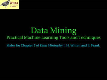
Robust regression “Robust” statistical method one thataddresses problem of outliersTo make regression more robust: Minimize absolute error, not squared errorRemove outliers (e.g. 10% of points farthest fromthe regression plane)Minimize median instead of mean of squares(copes with outliers in x and y direction) Finds narrowest strip covering half the observationsData Mining: Practical Machine Learning Tools and Techniques (Chapter 7)25
Example: least median of squaresNumber of international phone calls fromBelgium, 1950–1973Data Mining: Practical Machine Learning Tools and Techniques (Chapter 7)26
Detecting anomalies Visualization can help to detect anomaliesAutomatic approach:committee of different learning schemes E.g. decision treenearest neighbor learnerlinear discriminant functionConservative approach: delete instancesincorrectly classified by all of themProblem: might sacrifice instances of smallclassesData Mining: Practical Machine Learning Tools and Techniques (Chapter 7)27
Combining multiple models Basic idea:build different “experts”, let them voteAdvantage: often improves predictive performanceDisadvantage: usually produces output that is very hard toanalyzebut: there are approaches that aim to producea single comprehensible structureData Mining: Practical Machine Learning Tools and Techniques (Chapter 7)28
Bagging Combining predictions by voting/averaging “Idealized” version: Simplest wayEach model receives equal weightSample several training sets of size n(instead of just having one training set of size n)Build a classifier for each training setCombine the classifiers’ predictionsLearning scheme is unstable almost always improves performance Small change in training data can make bigchange in model (e.g. decision trees)Data Mining: Practical Machine Learning Tools and Techniques (Chapter 7)29
Bias variance decomposition Used to analyze how much selection of anyspecific training set affects performanceAssume infinitely many classifiers,built from different training sets of size nFor any learning scheme, Bias expected error of the combinedclassifier on new dataVariance expected error due to theparticular training set usedTotal expected error bias varianceData Mining: Practical Machine Learning Tools and Techniques (Chapter 7)30
More on bagging Bagging works because it reduces variance byvoting/averaging Note: in some pathological hypothetical situations theoverall error might increaseUsually, the more classifiers the betterProblem: we only have one dataset!Solution: generate new ones of size n by samplingfrom it with replacementCan help a lot if data is noisyCan also be applied to numeric prediction Aside: bias variance decomposition originally onlyknown for numeric predictionData Mining: Practical Machine Learning Tools and Techniques (Chapter 7)31
Bagging classifiersModel generationLet n be the number of instances in the training dataFor each of t iterations:Sample n instances from training set(with replacement)Apply learning algorithm to the sampleStore resulting modelClassificationFor each of the t models:Predict class of instance using modelReturn class that is predicted most oftenData Mining: Practical Machine Learning Tools and Techniques (Chapter 7)32
Bagging with costs Bagging unpruned decision trees known to producegood probability estimates Where, instead of voting, the individual classifiers'probability estimates are averaged Note: this can also improve the success rateCan use this with minimum expected cost approachfor learning problems with cost
Data Mining: Practical Machine Learning Tools and Techniques (Chapter 7) 5 Scheme independent attribute selection Filter approach: assess based on general characteristics of the data One method: find smallest subset of attributes that separates data Another method: use different learning scheme e.g. use attributes selected by C4.5 and 1R, or coefficients of linear