WIXLIB

138x 10Rel. Error along y 176140518041006020322021000.20.40.60.81xFigure 1: Relative error near the y 1 boundary for varying grid sizes when there is a change in boundarycondition type at x 0.5 from Neumann to Dirichlet.Similarly, for the Poisson equation in polar coordinates (r, φ) given by1 2u 2 u 1 u f (r, φ), r 2r rr 2 φ2(2.7)the approximate solution is given by ui,j u(rj , φi ), i 1, . . . , L, j 1, . . . , M . The resultingdiscretization is given by!!!2rj2ui,j ui,j 1ui,j 1 ui,j 1ui,j 1 ui,j 2rjhrj hrj 1hrhrj 1hrk hrj 1! j!(2.8)ui 1,j ui,j2ui,j ui 1,j2 rj fi,j . hφi hφi 1hφihφi 1Finally, in spherical coordinates (ρ, θ, φ), where θ is azimuthal angle and φ is a polar angle, thePoisson equation has the form 1 2u1 u12 u f (ρ, θ, φ).(2.9)ρ sinθ 2ρ2 ρ ρρ2 sin θ θ θρ2 sin θ φ2the approximate solution is given by ui,j,k u(ρk , θj , φi ), i 1, . . . , L, j 1, . . . , M , k 1, . . . , N .The discretized version of PDE (2.9) is given by!!ui,j,k 1 ui,j,k ui,j,k ui,j,k 12ρ2k sin2 θ hρk hρk 1hρkhρk 1!ui,j,k 1 ui,j,k 1 2ρk sin2 θhρ hρk 1!! kui,j 1,k ui,j,k ui,j,k ui,j 1,k2 sin2 θ(2.10) hθj hθj 1hθjhθj 1!ui,j 1,k ui,j 1,k sin θ cos θhθ hθj 1! j!ui 1,j,k ui,j,k ui,j,k ui 1,j,k2 ρ2k sin2 θfi,j,k . φφφφhi hi 1hihi 1

2.3Singularity Points in Polar and Spherical DomainsIn polar and spherical domains, the finite difference formulas for the Laplacian cannot be directly used for internal domain domain points corresponding to zeroes of the Jacobians J2 D(x, y)/D(r, φ) r and J3 D(x, y, z)/D(ρ, θ, φ) ρ2 sin θ.In particular, for the polar and spherical domains, a breakdown occurs at points with r 0(ρ 0). In the spherical domain, another breakdown occurs for points where θ {0, π}. Asolution to this problem is found by recalling to the definition of the Laplacian as the divergenceof the gradient. Using the fact that the divergence of a vector field q R2 or w R3 is given by,respectively,ZZZ11div q lim(q · n) dℓ, div w lim(w · n) dS,(2.11)S 0 S SV 0 V Vone can derive formulas that correctly approximate the Laplacian for points where the Jacobian issingular. In particular, in polar coordinates at r 0 with a variable step-size mesh, (2.11) yieldsa finite-difference relation! r 2NφNφ φXhφi hφi 1hi hφi 1 Xh1f (0, φ)(2.12) u2,j πu1,j242j 1j 1determining the value of u in the center of the disk. Note that conditionsu1,1 u1,2 . . . u1,L(2.13)must be added because the center value is independent of the polar angle φ. Also, hφi 1 hφNφPNφ hφi hφi 1when i 1. [Note that j 1 2π.]2For spherical coordinates at r 0, the divergence of the gradient yields, 1 L MXX(ui,1,2 ui,1,1 ) A′1 (ui,M,2 ui,M,1 ) A′Mui,j,2 Aui,j,1 A V f (0, θ, φ) rrh1h1hr1i 1 j 2(2.14)where A hr124 V π3 2 1 rh2 1hθj hθj 12 3!hφi hφi 12!sin θj , A′1,M 2π hr12 1 coshθ1,M2!!,,and the value of u at the origin is θ- and φ-independent:ui,j,1 u1,1,1 ,i 1, . . . , L;j 1, . . . , M.(2.15)Finally, for spherical coordinates at θ 0, the divergence of the gradient yields,ui,1,kSup Sdown rhrkhk 1!Nφui,1,k 1 Sup ui,1,k 1 Sdown X hrkhrk 1i 1 ui,2,k ui,1,k gg f (r, θ, φ) Ai Vrk hθ1(2.16)

whereSup hr 2π rk k2 2 1 cos hθ12 ,Sdown hr 2π rk k 12! θ hrk hrk 1hφi hφi 1h1rrghk hk 1 sin, Ai rk 442#" θ r 3 r 3hhh12πkkg rk V 1 cos.rk 3222 2 1 cos hθ12 , [For θ π, the expressions are the same, with ui,1,q ui,M,q , ui,3,q ui,M 2,q , and hθ1 hθM .]2.4Matrix StructureWe now illustrate the matrix structure arising from an application of finite-difference discretizationof the mixed Poisson BVP (1.2) in Cartesian and polar coordinates in two dimensions, and sphericalcoordinates in three dimensions.In two dimensions, for all points of a rectangular domain or a disk except for the center of the disk,the discretization of the Poisson equation as well as Dirichlet and Neumann boundary conditionsat any point indexed by (i, j) can be written in a general formaui,j bui 1,j cui 1,j dui,j 1 eui,j 1 Fi,j(2.17)with the appropriate choice for coefficients a, b, c, d, and e. Here Fi,j fi,j for internal meshpoints; it also includes terms associated with functions vD (x) or vN (x) at boundary mesh points.In Cartesian coordinates, the discretization yields a system of linear algebraic equations (LAE)containing N LM equations. In order to write equations (2.17) in the matrix formAu b,(2.18)one needs to re-index the matrix of unknown approximate values ui,j into a vector of length N ;this is done according to the formulau [u1,1 , . . . , uL,1 , u1,2 , . . . , uL,2 , . . . , u1,M , . . . , uL,M ]T .(2.19)Similar operations are performed for polar and spherical coordinates in order to bring the linearsystem to the form (2.18).Each one-dimensional discretization yields a tridiagonal matrix A1 , the discretization in two dimensions yields a block-diagonal matrix A A2 which consists of matrices A1 on the main diagonal,with additional layer-interaction elements (two extra nonzero diagonals), illustrated clearly in Figure 2 (left). [The three matrix structures shown in Figure 2 were observed using the Matlab spyfunction.]For a two-dimensional disk domain in polar coordinates, the matrix structure is rather similar,with the addition of singularity conditions (2.12), (2.13) which produce extra relations seen as ahorizontal and a vertical bar in the matrix plot in Figure 2 (middle).Similarly, in three dimensions (spherical coordinates), the corresponding matrix A A3 is ablock-diagonal matrix with A2 -type blocks on the main diagonal and two additional nonzero layerinteraction diagonals. The matrix structure is shown in Figure 2 (right); it also involves horizontaland vertical bars corresponding to relations (2.14), (2.15), and (2.16) at singular mesh points.Since the number of nonzero matrix entries depends on the number of unknowns linearly, and thematrix size – quadratically, the matrix structures become increasingly more sparse as the number

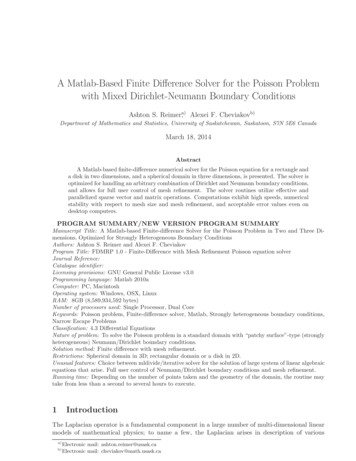
Figure 2: Left: matrix structure for a 9 9 Cartesian domain. Middle: matrix structure for a 9 9 polardomain. Right: matrix structure for a 6 6 6 spherical domain. [In each caption, nz stands for the numberof nonzero matrix elements.]of mesh points increases. It is therefore paramount that one utilizes a matrix solver that is efficientin solving (2.18) with large sparse matrices.Another important characteristic of the A matrix that needs to be discussed is the conditionnumberκ(A) kAk · kA 1 k,where kAk is some matrix norm. The condition number is commonly viewed as an upper bound ofthe error amplification coefficient for the problem (2.18), according to the formula kδAk kδbkkδxk κ(A) ,kxkkAkkbkwhere δA and δb are errors (resulting from roundoff and/or truncation errors) in the matrix andthe right-hand side, and δx is the resulting error in the solution.For matrices of the structure described above, condition numbers computed using the 1-normcan reach the order of 105 1010 , growing with the number of mesh points. An example of acomputation of relative errors and condition numbers for a Cauchy problem in a unit square withexact solution u(x, y) exp[ 300((x 0.45)2 (y 0.61)2 ) is given in Fig. 3, where calculationshave been performed for increasing numbers of points N in each direction, with no mesh refinement.The condition numbers were computed using Matlab condest 1-norm condition number estimate.The high matrix condition numbers do not provide limitations for the numbers of mesh points inthe computations, since a significantly more severe limitation is provided by memory constraints.Matrix condition numbers cannot be improved by preconditioners for the main mldivide routinesince it is based Gaussian elimination; for the iterative solver, the LU-decomposition is used as apreconditioner.2.5Matlab and Matrix Optimized CodeWith Matlab’s optimized routines for handling and solving linear matrix equations (2.18), includingvery large sparse matrices, it was an obvious choice to minimize the amount of programming effortrequired to develop this solver. By building a finite difference algorithm that avoids for-loops andtakes advantage of processor-specific fast vector operations implemented in Matlab, computationtime was dramatically decreased.

1101010910810 3107κ(A)Max. Relative Error 21010 410610Max. Relative ErrorConditon number 5102004006008001000510NFigure 3: Condition number and maximum relative error values versus the number N of mesh points ineach direction, for the Cauchy problem for a Possion equation in a unit square, with a known analyticalsolution. Black curves correspond to data obtained using mldivide; red dots indicate cases when an iterativesolver was used. Computations were performed for increasing values of N until memory limits were reachedfor the Matlab condest routine.With multi-core processor computers becoming the norm, Matlab has developed its vectorhandling routines to be parallelized across multiple cores, thus further decreasing the computationaltime required to obtain a solution. In particular, run examples discussed in the current paper weretested on a quad-core Intel processor, and in the course of the solution, the computational loadwas approximately equally distributed between the four cores.2.6Mesh RefinementFor some problems of the type (1.2), it may be necessary to employ mesh refinement. In particular,MFPT problems (1.1) involved small boundary traps (Dirichlet domains) that needed to be adequately resolved, with at least 100 mesh points per trap. At the same time, with common desktophardware limitations of standard laboratory computers, it was only possible to employ N 106data points, depending on the domain geometry. For example, for a unit square, computationswere performed with L M 1300; for a unit sphere, values around L 250, M N 100 wereused.Within the routines presented in the current paper, the refinement is done by applying a nonlinear scaling to the numerical mesh in any or every chosen direction, such that mesh points areconcentrated around expected regions of interest.An advantage gained by using the above mesh refinement procedure in terms of computing timeand accuracy can be illustrated by the following example. Consider an exact sharp-spike typesolution5 [(x 0.5)2 (y 0.5)2 ]u(x, y) e 10(2.20)and its corresponding Dirichlet problem for the Poisson equation in the unit square. Since the spikeis located at the square center, a cubic refinement curvex̃ 4(x 0.5)3 0.5is used in both spatial directions. Fig. 4 shows the maximum relative error for the numerical solutionwith mesh refinement with a mesh size of 100 100 and the maximum error for the solution withoutmesh refinement on an N N mesh, as well as the the amount of time required to compute eachsolution. The error level of the solution using a mesh with N 100 and mesh refinement is reached

1200.815Max. Relative 0400450500Computation time (s)Max. Relative ErrorComputation time0550NFigure 4: Left: the mesh refinement curve used for both x- and y-directions. Right: comparison of maximumrelative error (dashed curves) and computational time required (solid curves) for solution with a 100 100mesh with mesh refinement (horizontal lines) and solutions using an N N mesh without mesh refinement,100 N 550.by a solution without mesh refinement only for N 520; the latter also requires significantly morememory and time.The requirement of mesh refinement is especially critical in the three-dimensional domain of theunit sphere. For example, for the MFPT problem with boundary conditions involving three traps(Dirichlet regions) centered at polar angles φ π/3, π, 5π/3 on the equator, the refinement curvesare shown in Fig. 5. Places of almost-zero slopes correspond to multiple points of a homogeneousmesh being concentrated near regions of interest. For the above spherical example, with L 250points in the polar φ-direction and M N 100 in ρ- and θ-directions, small Dirichlet (trap)boundary regions we resolved at 9 points per trap when no mesh refinement was used, and at 799points per trap when mesh refinement shown in Fig. 5 was applied.10.80.60.4Polar angleAzimuthal angleRadius0.2000.20.40.60.81Figure 5: Mesh refinement for a sphere with regions of interest centered at polar angles φ π/3, π, 5π/3 onthe equator. The horizontal axis corresponds to input (homogeneous) mesh and the vertical axis correspondsto output (refined) mesh.Several run examples using mesh refinement in two and three dimensions are presented in thesections below.It is important to note that the mesh refinement algorithm used in the current work is not a localrefinement; in fact, the refinement propagates through the domain, which yields extra points, orpoints that appear to have no function (see, e.g., left plot in Fig. 7, and upper left plot in Fig.10). Variants of finite-difference methods that used only local mesh refinement were considered by

the authors. It was however found that even though the number of points in local mesh refinementalgorithms is smaller, computations in fact take significantly longer, due to the fact that a localfinite-difference refinement patch destroys the block matrix structure discussed in Section 2.4.Hence the current (somewhat nonlocal) mesh refinement algorithm was adopted as an efficient onefrom the practical point of view.3Rectangular Domain in Two DimensionConsider a mixed Poisson problem (1.2) for the rectangular domain Ω {(x, y) 0 x Lx , 0 y Ly }. Denote the numbers of mesh points in x- and y-directions by L and M , respectively.3.1Program SequenceIn order to numerically solve the problem (1.2) for a rectangle in cartesian coordinates, one needsto perform the following steps.1. Create a new folder and copy all files of some example that solves the Poisson equation in arectangle into that new folder.2. Modify the file forcing.m: change the line f mat(i,j) Q where Q(xi , yj ) is the desiredforcing function.3. Modify the file dirichlet boundary.m: change the if-conditions as needed, and change thelines diriBC(i,j) Q so that Q vD (xi , yj ) specifies the desired Dirichlet boundary conditionof the problem (1.2).4. Modify the file neumann boundary.m: change the if-conditions as needed, and change thelines neuBC(i,j) Q so that Q vN (xi , yj ) specifies the desired Neumann boundary conditionof the problem (1.2).5. Modify the files x refine function.m and y refine function.m to introduce necessarymesh refinement. The input parameter in is a vector that will contain homogeneous meshpoints; the output parameter out has to either equal in (no mesh refinement) or a functionthat acts on in to concentrate/rarify mesh where needed. Each refinement function must bea monotone increasing function. It is the user’s responsibility to satisfy the conditionsin(1) out(1),in(end) out(end)(3.1)in order to preserve the square side lengths.[Often it is useful to plot out as a function of in using Matlab plot(in, out), to obtain acurve similar to those in Fig. 5.]6. Run the solver routine:[xs ys v relres iter resvec] rectangle 2d poisson(x max,y max,num xs,num ys,’x refine function’,’y refine function’,’dirichlet boundary’,’neumann boundary’,’forcing’,useiter)where x max and y max are the domain sizes Lx , Ly in the x-and y-directions respectively;num xs and num ys are the numbers of mesh points L, M in the corresponding directions;x refine function.m and y refine function.m are the filenames of external Matlab functions for mesh refinement; dirichlet boundary.m and neumann boundary.m are the filenames of external Matlab functions that generate the Dirichlet and Neumann boundary conditions; forcing.m is the name of an external Matlab function that generates the forcing

term at every point of the domain; useiter is an optional parameter (default value 0) which,if set to a nonzero value, forces the solver to use an iterative method to solve the sparse linearsystem.Details about the parameters passed to the rectangle 2d poisson solver, in particular,formats of the external functions, are discussed below within the run examples (Section 3.2).The normal output of the solver consists of a matrix of approximate solutions v of the problem(1.2) at mesh points stored in matrices xs and ys. The solution is ready for plotting usingthe routinesurf(xs,ys,v);When the parameter useiter is set to a nonzero value, an iterative solver for a linear sparsesystem is used, and the output values relres, iter and resvec are the final residual, thenumber of iterations used, and a vector of the history of the residuals, respectively.Remark 3.1. The solver applies the following rules to determine which boundary condition to useat each boundary point. If at a given boundary point, a Dirichlet boundary condition is specified, then it is used, andthe Neumann boundary condition is ignored (if specified at all). If at a given boundary point, a Neumann boundary condition needs to be specified, the valueprovided for diriBC for that point in the file dirichlet boundary.m must be set to NaN.The above rules let the user avoid duplicating if-conditions when the problem involves a mixtureof Dirichlet and Neumann boundary parts.3.23.2.1Run ExamplesExample R1As a first run example for the mixed Poisson problem (1.2) for a rectangular domain, we letLx 1, Ly 2, with L M 100 mesh points in each direction, and no mesh refinement.We define the solution v(x, y) to be a known “chair-shaped” function given by v(x, y) 3 exp{ 100(x 0.95)2 10(y 1)2 } 1 cos [2π(y 1)(x 0.5)] .(3.2)Suppose the function (3.2) solves the problem (1.2) with Neumann boundary conditions at x 0and y 0, and Dirichlet boundary conditions at x 1 and y 1. The boundary conditions vN andvD and forcing f (x, y) are computed by substituting the expression (3.2) into the problem (1.2).The Matlab files for the boundary conditions, forcing, and mesh refinement functions are givenin Appendix A.The solver is run by the command[xs ys v relres iter resvec] rectangle 2d poisson(1, 2, 100, 100, ’x refine function’,’y refine function’,’dirichlet boundary’,’ne

Department of Mathematics and Statistics, University of Saskatchewan, Saskatoon, S7N 5E6 Canada March18,2014 Abstract A Matlab-based finite-difference numerical solver for the Poissonequation for a rectangle and a disk in two dimensions, and a spherical domain in three dimensions, is presented. The solver is