WIXLIB

E. Trutnevyte / Energy 106 (2016) 182e193scenarios seem more probable that the ones that have not beenshown in detail [31]. As a result, there has been an increasing interest in model evaluation to assess the performance of models, cf.[32]. One of the unresolved critiques is the use of cost optimization[25]. This papers aims to assess the adequacy of cost optimizationfor modeling energy transitions.Ever since the first bottom-up energy system models weredeveloped, there has been a tension between exploratory andpredictive use of energy scenarios. Nowadays modelers frame energy scenarios resulting from the models as possibilities whatmight happen and not predictionsdthat is, as scenarios “for insights, not numbers” [p. 449, 33]. But whether used for predictionsor insights, scenarios generated with models are implicitlyassumed to be able to give some indication of what is possible inthe future and, in this way, are implicitly used as proxies of thefuture. From the multidimensional space of possible futures that isdefined by technical, economic, environmental and other constraints, bottom-up models use cost-optimization to narrow downthis space to one scenario to analyze further. But even intuitivelyone senses that real-world energy system transition may not becost optimal. To date the bottom-up modeling community has beenstruggling to make the bridge between the need for scenarios thatare reasonable proxies of the real-world transition and the modelsthat cannot provide such proxies.With the aim to resolve the aforementioned tensions and lack ofex-post evidence in bottom-up energy system models, this papergathers historic evidence and conducts an ex-post modeling exercise in order to understand whether cost optimization approximates the real-world energy transition. The UK electricity systemfrom 1990 to 2014 is modeled, using bottom-up electricity systemmodel D-EXPANSE. With hindsight, the actual (real-world) transition is known and can be compared to the modeled cost-optimalscenario. As historic data on the model parameters, such as technology and fuel costs, are collected, the parametric uncertainty canbe nearly eliminated in order to enable exploration of the costoptimization rationale. Due to its ex-post modeling approach, thisstudy is the first of its kind.This paper is structured as follows: Section 2 provides an overview why cost optimization is used in bottom-up energy systemmodels and why it may be limited; Section 3 introduces the bottomup energy system model D-EXPANSE; Section 4 describes the caseand data of the UK electricity system transition in 1990e2014;Section 5 presents the ex-post modeling results; Section 6 discussesthe results and proposes future research needs; Section 7 lists theimplications for modeling the future energy transition with bottomup energy system models; and Section 8 concludes.2. Rationale for cost optimization and its limitationsCosts are among the key drivers of the energy system transition.On this basis, there are two interlinked arguments why cost optimization is used in bottom-up energy system models: the socialplanner's approach and the partial equilibrium argument. The social planner's approach originates in planning and public policy andassumes that there is a single decision maker, who aims atachieving the best outcome for the society as a whole. Such anoutcome is reached by maximizing the sum of the energy supplier'sand consumer's surpluses in the case of elastic demands. Thissurplus maximization is transformed into an equivalent of minimization of the total system costs that represent the negative of thesurplus [12]. With fixed demands, only the total costs for suppliersare minimized. In reality, however, such a single social planner doesnot exist and, especially after market liberalization, multipleinteracting energy suppliers and consumers with heterogeneousdecision powers and stakes shape the energy transition [30].183The partial equilibrium argument assumes that energy supplydemand equilibrium is reached, when the total surplus, as in thesocial planner's approach, is maximized [12]. However, the generalequilibrium assumption is not shared by institutional and evolutionary economists [34], while the partial equilibrium assumptiondoes not account for the interaction between the analyzed sectorand the wider economy.In addition to these critiques of both the social planner's andpartial equilibrium arguments, the heterogeneous actors in the realworld do not always act rationally as assumed in models [35,36]and, if they do, there are other factors than only costs that theymay consider [37]. Decision may be made using the principle ofsatisficing rather than optimizing, especially in face of multiplestakes. Energy transition is actively shaped by policy makers andother decision makers, who in the process require several alternatives to consider and choose from [15,38,39]. Neither posing onecost-optimal alternative for discussion nor expecting that it will beprescriptively followed is realistic. After all, the energy system ishighly complex and it cannot be steered to a single least cost stateanyway [40].In light of such critiques, the bottom-up energy systemmodeling community has attempted to improve the models todeviate from cost optimal scenarios under perfect foresight to theones that are believed to be more realistic. Such attempts includethe myopic instead of perfect foresight versions [41], multiobjective optimization [42], analysis of parametric uncertainty[43,44], inclusion of external costs in addition to direct costs [45],models of multifaceted nature of behavior and decisions [30,46],second-best policy scenarios [47], near-optimal scenarios[39,48e50], or modeling constraints that enforce the deviationfrom cost optimality [51]. In addition, simulation rather than costoptimization models have been developed. Simulation models relyon historic evidence or theory-informed description of model variables to simulate the future scenarios, e.g. [52].Even if ex-post validation and broader evaluation of models hasbeen repeatedly called for [27,53], the handful of existing studiescompared past scenarios and real-world transition on a genericlevel [17,23,26,27,31,54,55]. With the exception of McConnell andcolleagues [56], no ex-post modeling studies exist that enableunpicking the reasons behind the mismatch of the modeled energyscenarios and the real-world transition. For example, such reasonscould be cost optimization, parametric assumptions, structural assumptions, model boundaries, or others.Recently, three-decades-old techniques [37,57] for exploringnear-optimal solutions of optimization tasks have been applied tobottom-up energy models [39,48e50]. All these studies haveshowed that a small deviation in total system costs leads to a verydiverse set of near-optimal energy scenarios. Keepin and Wynne[18] have already pointed out to this limitation of bottom-up energy system models, when small differences in input parameters,such as technology costs, cause large differences in solutions. Suchlimitation may not be resolved by multi-objective optimization. Forexample, Hara [50] has conducted vehicle mix optimization usingtwo objectives of carbon emissions and costs. The resulting Paretooptimal solutions are less diverse than the near-Pareto optimalsolutions, i.e. solutions that have up to 0.5% higher emissions (orcosts) as compared to their respective Pareto optimal solution. Insum, the use of optimization tends to gloss over the diversity inpossible near-optimal energy scenarios.Even if the real-world energy system may not evolve in a costoptimal way, costs are still among the key drivers. It is thusmeaningful to assume that the energy system will not evolve in themost expensive and irrational way. Instead, the real-world transition will likely be somewhere close to the cost-optimal scenario,but not necessarily exactly the optimal one. Several modeling

184E. Trutnevyte / Energy 106 (2016) 182e193studies, with bottom-up or other types of models, allowed higherthan optimal system costs in energy scenarios, e.g. a deviation of10e30% in total system costs [39,48e50,58,59]. However, there islittle evidence of what level of deviation from cost-optimality couldbe adequate. Empirical evidence from interviews in Switzerland,reported by Trutnevyte and colleagues [60], showed that variousstakeholders would accept 30% higher total system costs if thesystem would reach other goals, e.g. related to environmentalconcerns or energy independence. This is the only existing evidence, but it originates in the stated preferences approach and thusmay also not be an adequate representation of the real world.3. D-EXPANSE modelIn order to understand whether cost optimization approximatesthe real-world energy transition, the D-EXPANSE model is used tomodel the UK electricity system transition from 1990 to 2014. According to the typology of Hourcade and colleagues [61], DEXPANSE (Dynamic version of EXploration of PAtterns in Nearoptimal energy ScEnarios) has the structure of the conventional,bottom-up, technology rich, cost optimization model with perfectforesight. Alternative typologies of bottom-up and top-downmodels exist [62]. D-EXPANSE is considered bottom-up because itdoes not have macro-economic completeness.In addition, D-EXPANSE has two state-of-the-art features. First,it systematically explores near-optimal energy scenarios[39,48e50]. Even with a single set of input assumptions, the modelproduces a wanted number of different scenarios that are eithercost-optimal or near-optimal. Near-optimal scenarios are scenarios,whose total system costs do not exceed the predefined upper limitthat is higher than the costs of the cost-optimal scenario. Second, inorder to understand the influence of the parametric uncertaintyMonte Carlo technique is used to sample sets of various inputs.Other existing models that explore near-optimal energy scenarios[39,48e50] have been limited to deterministic versions and, in linewith the wedges approach [63], modeled only one single year in thefuture. D-EXPANSE thus substantially extends the current models.It models the transition from today to the future rather thanadopting the wedges approach and it conducts Monte Carlo runs toaddress parametric uncertainty. D-EXPANSE complements otherversions of the EXPANSE model that adopted wedges approach[39], was spatially explicit [49], and included optimization of otherobjectives beyond costs [64].Fig. 1 summarizes the procedure that is used for the ex-post UKelectricity system modeling. D-EXPANSE and its mathematicalformulation are introduced in detail in Appendix A. In brief, thedeterministic D-EXPANSE run and Monte Carlo runs are conductedin parallel in order to compare them for better understanding of therole of parametric uncertainty. D-EXPANSE is at first run in costoptimization mode to find the least cost solution (scenario), under aset of supply-demand, technology and resource constraints. Then,the total system costs of the cost-optimal scenario are evaluatedand used as the anchor point for generating the near-optimal scenarios. The maximum deviation, called slack and expressed as(Cnear-optimal Coptimal)/Coptimal, is allowed from the total costs of thecost-optimal scenario. Costs then become a constraint and not theobjective function in D-EXPANSE. The technique of efficientrandom generation [37,57] is used to produce 500 scenarios that allmeet the model constraints and do not exceed the total systemscosts plus the slack. The cost-optimal and near-optimal scenariosare then compared to the real-world UK electricity system transition, for which the historical data are available. In Monte Carlo runsthe randomly drawn technology costs, electricity demands andsome technology parameters also produce variation in the realworld transition and its costs.The large ensembles of cost-optimal and near-optimal scenariosare then analyzed for additional insights. There are 501 scenarios(one cost-optimal and 500 near-optimal scenarios) in the set of thedeterministic D-EXPANSE run and 250'500 scenarios in the MonteCarlo version (501 optimal and near-optimal scenarios times 500Monte Caro runs). These large ensembles are analyzed usingdescriptive statistics and scenario visualization. Nine maximallydifferent scenarios, which differ from each other in installed capacity per technology as much as possible, are extracted fordetailed inspection using the adapted distance-to-selected technique [49,65].D-EXPANSE has a rather stylized reference energy system, butwith all its essential elements. Such a stylized representation is anadvantage for reducing the computing time of thousands of modelruns and for clarity, when extracting patterns from the large anddiverse ensembles of near-optimal scenarios. D-EXPANSE modelsthe electricity generation mix, electricity import through interconnectors and pumped hydropower storage to supply the UKelectricity demand. The electricity demand is exogenously assumedin line with the historic data and is not modeled as elastic. Theelectricity dispatch is based on three-stage load curve, includingbaseload, shoulder and peak loads. Transmission and distributionare not modeled and these losses are included as exogenous assumptions, since D-EXPANSE is not spatially explicit and thuscannot account for transmission and distribution costs and efficiency differences due location of power plants. Technology costsare assumed exogenously too in line with the historic data; technology learning effects are not endogenously modeled.4. UK electricity system transition in 1990e2014 and themodel input dataThe D-EXPANSE model was used to model the UK electricitysystem transition from 1990 to 2014 (five time steps of 5 years).Since energy system modeling activities have been shown to mirrorthe policy discussions of their time [23,66], discussions from early1990s were used to set up the model. The UK Energy Act 1983 andsubsequent White Paper 1988 initiated the privatization process inthe UK electricity sector. This privatization was completed in 1991,whereas the subsequent six years were spent “in search of the fulldiscipline of the market” [p. 12, 67] until the market was fullyopened to competition in 1999. With this aim to open the marketthat was previously dominated by coal, oil and nuclear power,policies targeted new market players, such as combined cycle gasturbines (CCGTs). After the oil crises in 1973 and 1979, beliefs thatoil prices were on the upward trend led to stronger focus on nonfossil fuel alternatives, such as renewable energy. For example,first commercial wind power park started operating in the UK in1991.The electricity generation technologies that are included in DEXPANSE are taken from the studies of early 1990s [23]. The annualsupplied electricity requirement, peak demand and baseload demand are available from statistics. Reconstruction of the historicalinvestment costs, operation and maintenance, and fuel costs haveproved to be the biggest challenge. While the fuel and investmentcosts are relatively easier to find [54,67], hardly any data is availableon the operation and maintenance costs. Thus, these costs areassumed as in various energy modeling studies in the 2000s.The modeling data and uncertainty ranges for Monte Carlo runsare summarized in Appendix B. Uniform distributions are used inMonte Carlo runs, because the aim is to understand the spectrum ofuncertainty rather than deliver probabilistic modeling outcomes.The D-EXPANSE runs are conducted for two discount rates: 3.5%and 8%. The rate of 3.5% is the social discount rate used in recent

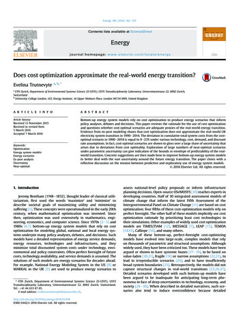
E. Trutnevyte / Energy 106 (2016) 182e193DeterminisƟc Cost-opƟmal scenario(1 scenario)run500 MonteCarlo runsCost-opƟmal scenario(1 scenario for everyMonte Carlo run)Near-opƟmal scenarios(500 scenarios; with slack)Near-opƟmal scenarios(500 scenarios for everyMonte Carlo run; with slack)Real-worldtransiƟon(1 scenario)Real-world transiƟon(1 scenario for everyMonte Carlo run)185Compare modeledscenario with thereal-world transi onFigure 2Figure 3Apply descrip vesta s cs methodsto 501 scenariosFigure 5Select9 maximallydifferent scenariosFigure 2Compare modeledscenarios with thereal-world transi onFigure 4Apply descrip vesta s cs methodsto 250500 scenariosFigure 6Figure 7Select9 maximallydifferent scenariosFig. 1. D-EXPANSE procedure for ex-post UK electricity system modeling.modeling and policy appraisal studies [68]. The rate of 8% was usedin the UK energy modeling studies in 1990s [69,70].In 1988 UK accepted the targets of European Union LargeCombustion Plant Directive (88/609/EEC), which aimed at limitingsulfur dioxide, nitrogen oxides and particle emissions. Implementation of this directive imposed emission reduction fromexisting power plants above 50 MW capacity as well as set apollution ceiling for new plants. In D-EXPANSE it is assumed that allnewly built plants are in line with the directive, because thepollution ceiling was mandatory for new plants. Since the retirement of existing plants is reconstructed from the historical statistics, it is assumed that existing plants either retire or arerefurbished to meet the directive's reduction requirements.In terms of greenhouse gas emissions, in 1990 Margaret Thatcherspoke to the Royal Society about climate change for the first time. In1992 UK signed the United Nations Convention on Climate Change atRio de Janeiro. However, the climate mitigation action had beenmaturing until 2008, when the Climate Change Act was released[67]. Although the period after 2008 is towards the very end of themodeled timeframe, atmospheric pollution policies and constraintsare not included in D-EXPANSE. But greenhouse gas emissions of thegenerated scenarios are calculated in order to gain insight on theinteractions between cost optimization and emissions.5. Ex-post modeling results5.1. Cost-optimal scenario vs. real-world energy transitionThe modeled cost-optimal scenario of the deterministic DEXPANSE model run with 3.5% discount rate is compared to thereal-world transition in terms of installed capacity in Fig. 2. Thecost-optimal scenario is not identical to the real-world transition.First, in the early 1990s the so-called ‘dash for gas’ happened in theUK, when gas CCGTs were rapidly deployed. In the modeled costoptimal scenario the ‘dash for gas’ happens to a lesser extent.Due to perfect foresight D-EXPANSE anticipates the gas price increase after 2000, related to the peak of the UK own gas productionin 2000 and the subsequent net import of gas after 2004. In the realworld neither policy makers nor investors have such perfectforesight. This lack of perfect foresight contributes to this difference between the modeled cost-optimal scenario and real-worldtransition. In fact, the real-world transition has been argued tofollow the most investable path rather than the path with thelowest total costs in the long run [71]. If real options thinking isadopted, then other management decisions, such as option to wait,commit to a follow-on investment. or abandon activity, are alsoconsidered.Winskel [72] explained the ‘dash for gas’ in the UK as a result of acombination of factors, such as electricity market liberalizationpolicies, resource availability, falling prices at the time, improvingturbine performance, atmospheric pollution legislation, and institutional tensions from the nationalization period. Pearson andWatson [67] argued that the primary cause for the ‘dash for gas’ wasthe policy to bring new players into market dominated by coal: “TheRECs [Regional Electricity Companies], wanting to limit the majorplayer's market power, contracted for electricity from CCGTs, partowned by RECs themselves and the oil companies. The regulator,keen to encourage new company entry to promote competition,allowed the RECs to include power purchase costs from IPPs [Independent Power Producers] in their regulated price caps and so, topass them through to costumers. This was a controversial decision eand was taken despite evidence that the new CCGTs could be moreexpensive than the plants they were replacing” [p. 12, 67]. Especiallythe last sentence shows that a deviation from the sole focus on costswas acceptable to achieve another objective of increasing the diversity of market players and fostering competition.Instead of CCGTs, the modeled cost-optimal scenario has ahigher share of new coal and nuclear power plants than the actualtransition. In reality, the construction of new nuclear plants wasunder debate in the UK at that time and thus delayed. Even thoughthe Government gave the green light to Sizewell B nuclear plant in1986, it was commissioned only in 1994 due to uncertain publicsupport and the debts of the nuclear industry. The estimates of thelevelized costs for nuclear electricity in 1990s were also higher thanthe estimates for gas CCGT, although the cost out-turns, in thesubsequent years dropped [54]. The deployment of new coal plantswas limited due to the aforementioned atmospheric pollutionregulations as well as due to the coal miners' strikes in 1984e1985,leading to more than a half of deep coal mines being closed by 1992.The indirect or lifecycle costs related to coal and nuclear, such as forair pollution or long-term nuclear waste storage, were notaccounted for in D-EXPANSE.After 2005 an increasing share of renewable electricity technologies has been deployed in the UK, as a result of stronger climatechange-related policies. Such tendency, however, is not reproducedin the modeled cost-optimal scenario because climate change

E. Trutnevyte / Energy 106 (2016) 182e1931006050201990Total installed capacity, GWTotal installed capacity, GW200020052010One maximally-different solution8004001005040405019901995200020052010One maximally-different solution0019901995200020052010One maximally-different 00020052010One maximally-different solution1200One maximally-different 000200520100One maximally-different solution200020052010One maximally-different 80150100150 1201000100150 120800One maximally-different solution400201990201020604020058010080200060150 12010019951008001990150 12020205020606010060150 120800100100120Total installed capacity, GW19951000802012001006040150Discounted costs, bnGBP(1990)10080One maximally-different solution150 1202010Discounted costs, bnGBP(1990)Total installed capacity, GW1000Real-world transition150 120Discounted costs, bnGBP(1990)Cost-optimal scenario120Discounted costs, bnGBP(1990)186Wind offshoreHydro storageWind onshoreImportNuclearWasteOil & otherBiomassGas CCGTLandfillCoalWave & TidalCumulative total costsSolar PVCumulative investment costsHydro RoR0Fig. 2. Comparison of the modeled cost-optimal scenario, real-world transition, and nine maximally-different near-optimal scenarios (deterministic run; 3.5% discount rate; 23%slack).policies and other atmospheric pollution constraints have not beenincluded. Due to its focus on costs, the cost-optimal scenario doesnot include costlier renewable technologies.Due to perfect foresight the model also anticipates the decline inelectricity demand after the economic crisis in 2008. The installedcapacity in the cost-optimal scenario thus decreases in the finaltime step. In the real-world transition, however, new capacities arebuilt. A large share of this new capacity are renewable energysources that have lower contributions to the peak equation andthus lead to a substantial difference between the total installedcapacity of the optimal scenario and the real-world transition.Fig. 3 compares the evolution of cumulative total system costs inthe case of the modeled cost-optimal scenario and the real-worldtransition. In order to make a consistent comparison, the costs ofthe real-world transition are evaluated using the same technologyand fuel costs and system boundaries as in D-EXPANSE. The costs ofthe real-world transition can be seen not to follow the cost-optimalpath. When 3.5% discount rate is used, the cumulative total systemcosts in 1990e2004 exceed the costs of the cost-optimal scenarioby 5% and in 1990e2014 e by 16%. When 8% discount rate is used,the deviation in 1990e2004 is 5% and in 1990e2014 e by 12%.In order to examine whether this deviation originates in parametric uncertainty in energy demand, technology data and costs,500 Monte Carlo runs are conducted for each case of 3.5% and 8%discount rates. The spread of deviations in 1990e2004 and1990e2014 are shown in Fig. 4. With both 3.5% and 8% discount

Cumulative discounted total system costs, bnGBP(1990)E. Trutnevyte / Energy 106 (2016) 182e1933% discount 8% discount rate1101000199018720002005Year2010Real-world transitionCost-optimal scenario01990199520002005Year2010Fig. 3. Comparison of the cumulative total system costs of the mod

predictive use of energy scenarios. Nowadays modelers frame en-ergy scenarios resulting from the models as possibilities what might happen and not predictionsdthat is, as scenarios "for in-sights, not numbers" [p. 449, 33]. But whether used for predictions or insights, scenarios generated with models are implicitly