Transcription
Downloaded from orbit.dtu.dk on: May 12, 2022The NNSYSID Toolbox - A MATLAB Toolbox for SystemNeural NetworksIdentification withNørgård, Peter Magnus; Ravn, Ole; Hansen, Lars Kai; Poulsen, Niels KjølstadPublished in:Proceedings of the 1996 IEEE Symposium on Computer-Aided Control System DesignLink to article, DOI:10.1109/CACSD.1996.555321Publication date:1996Document VersionPublisher's PDF, also known as Version of recordLink back to DTU OrbitCitation (APA):Nørgård, P. M., Ravn, O., Hansen, L. K., & Poulsen, N. K. (1996). The NNSYSID Toolbox - A MATLAB Toolboxfor System Identification with Neural Networks. In Proceedings of the 1996 IEEE Symposium on ComputerAided Control System Design (pp. 374-379). IEEE. https://doi.org/10.1109/CACSD.1996.555321General rightsCopyright and moral rights for the publications made accessible in the public portal are retained by the authors and/or other copyrightowners and it is a condition of accessing publications that users recognise and abide by the legal requirements associated with these rights. Users may download and print one copy of any publication from the public portal for the purpose of private study or research. You may not further distribute the material or use it for any profit-making activity or commercial gain You may freely distribute the URL identifying the publication in the public portalIf you believe that this document breaches copyright please contact us providing details, and we will remove access to the work immediatelyand investigate your claim.
Proceedingsof the 1996 IEEE International Symposiumon Computer-Aided Control System DesignDearborn, MI September 15-18,1996TA01 10:20Xtisn with NesM. N@rgaard*,0. Ravn*, L.K. Hansen**,N.K. Poulsen***Department of Automation, building 326. pmn, or@iau.dtu.dkDepartment of Mathematical Modelling, building 32 1. nkp, lkh @imm.dtu.dkTechnical University of Denmark (DTU), 2800 Lyngby, Denmark**network toolbox [ 2 ] .Although a small overlap with this hasbeen unavoidable the two toolboxes are, however, fundamentally different. While the Neural Network toolbox hasbeen designed for covering a variety of network architectures and for solving many different types of problems, theNNSYSID toolbox is specialized to solve system identification problems. Because the overlap is limited we havetherefore chosen to develop NNSYSID completely independent of the Neural Network toolbox.AbstractTo assist the identification of nonlinear dynamic systems, aset of tools has been developed for the MATLAB” environment. The tools include a number of different modelstructures, highly effective training algorithms, functionsfor validating trained networks, and pruning algorithms fordetermination of optimal network architectures. The toolbox should be regarded as a nonlinear extension to theSystem Identification Toolbox provided by The MathWorks, Inc [9]. This paper gives a brief overview of theentire collection of toolbox functions.All toolbox functions have been written as “m-functions,”but some CMEX dublicates have been coded for speedingup the most time consuming functions. The only officialMathworks toolbox required is the Signal ProcessingToolbox.1. IntroductionInferring models of dynamic systems from a set of experimental data is a task which relates to a variety of areas.Technical as well as non-technical. If the system to beidentified can be described by a linear model quite standardized methods exist for approaching the problem. Furthermore, a number of highly advanced tools are availablewhich offer assistance in solving the problem 191. When itis unreasonable to assume linearity and if the physical insight into the system dynamics is too limited to propose asuitable nonlinear model structure, the problem becomesrelatively complex. In this case some kind of generic nonlinear model structure is required. A large number of suchmodel structures exist, each characterized by having different advantages and disadvantages. The multilayer perceptron neural network [7] has proven to be one of the mostpowerful tools in practice and thus it has been selected asthe key technology in our work. The attention has beenrestricted to networks with a single hidden layer of tunh (orlinear) units since these offer a satisfying flexibility formost practical problems. MATLAB 4.2 has been chosen asthe environment in which to operate due to its popularity,the simple user-interface, and its excellent data visualization features. The Mathworks, Inc already offers a neuralThe NNSYSID toolbox has primarily been designed from acontrol engineering perspective, but can be used for manyother applications. For example is time series analysis alsosupported (i.e. no exogenous variablekontrol signal). Thetoolbox is mainly created for handling Multi-Input-SingleOutput systems (with possible time delays of different order). Identification of multi-output systems is only supported for the most common model structures.A number of demonstation programs have been implemented with the GUI facilities of MATLAB 4.2. These aredesigned to give a quick introduction to the toolbox anddemonstrates most of the functions. The toolbox is alsoaccompanied by a “MATLAB style” manual, which fullydocuments the entire collection of functions [ 111.The outline of the paper is as follows: first a brief recapitulation of the basic identification procedure is given andsubsequently the toolbox functions are presented by category in accordance with the overall identification procedure.394Authorized licensed use limited to: Danmarks Tekniske Informationscenter. Downloaded on March 02,2010 at 07:30:10 EST from IEEE Xplore. Restrictions apply.
network, and j(tl6) Y(tlt - I,@ denotes the one-stepahead prediction of the output.2. The Basic ProcedureFig. 1 shows the procedure usually followed when identifying a dynamic system. Prior to the execution of the procedure two issues should be considered: what a priori knowledge about the system is available and what is the purpose(i.e., the intended application of the model)?. Typically,these issues will have a strong impact on the entire procedure.NNARX structure.ti( ) g(cp(t),13) and.q(O [y(t-1)u(t-n,)y(t-n,).u(t-n,-n, l)]7NNOE structure. i(tl8) g(q(t) ) andF - - 1----I. jyt - n,,le)7u ( t - n , ) . u ( t - n , -nk 1)]NNARMAXI structure. j(t(8) g(q,(t),8) C(q-')&(t)q(t) [ j ( t- lie)ODEL STRUCTU.q(t) [q:(t) &(I-1)ESTIMATE. [y(t-l) (t-n,)&(t-n')ITy(t-nu).u ( t - n , -n, 1)&(t-1). ( t - n , f ( tis) the prediction error: ( t )y ( t ) - jl(tl8) and C isa polynomial in the delay operator:C(q-1) 1 clq-1 . cnrq-"'Figure 1. The system identijkation procedure.It is assumed that experimental data describing the underlying system in its entire operating range has been obtainedin advance with a proper choice of sampling frequency:NNARMAX2 structure. i(tl6) g ( q ( t ) , 8 ) andqw [ Y W )ZN ([u(t),y(t)]It l,.,N]***u(t-n,)U(?) specifies the input to the system while y ( t ) specifies theoutput.y(t-n,)u ( t - n , -n, 1 ).&(t-1).&(t-n,)ITNNSSIF structure (state space innovations form). h e dictor:The toolbox is designed to cover the remaining three stagesas well as the paths leading from validation and back toprevious stages. The following chapters will briefly describe the functions contained in the toolbox. 1) g ( q ( t ) , e )j(tl8) C(8)i(t)3. Selecting a Model StructurewithAssuming that a data set has been acquired the next step isto select a set of candidate models. Unfortunately, this ismuch more difficult in the nonlinear case than in the linear.Not only is it necessary to choose a set of regressors, but anetwork architecture is required as well. The implementedmodel structures more or less follow the suggestions givenin [15]. The idea is to select the regressors as for the conventional linear model structures and then, afterwards, determine the best possible neural network achitecture withthe selected regressors as inputs.To obtain an an observable model structure, a set ofpseudo-observability indices must be specified just as in[SI.For supplementary information see chapter 4,appendixA in [8].0NNZOL structure (Input-Output Linearization).i(tl@ f ( Y @ - I), .,y(t -nu ,u(t - 2), ,.,u(t - nh 1,e f l g(y(t - I),. .,y ( t - n,),u(t - 21,. .,u(t - n,),B,)u(tThe toolbox provides the six model structures listed below.dt)is the regression vector, 8 is the parameter vector containing the weights, g is the function realized by the neural- 1)f and g are two separate networks. This structure differsfrom the previous ones in that it is not motivated by a linear375Authorized licensed use limited to: Danmarks Tekniske Informationscenter. Downloaded on March 02,2010 at 07:30:10 EST from IEEE Xplore. Restrictions apply.
model structure. NNIOL models are particularly interestingfor control by input-output linearization.1 -OTDO2NFor NNARX and NNIOL models there is an algebraic relationship between prediction and past data. The remainingmodels are more complicated since they all contain a feedback from network output (the prediction) to network input. In the neural network terminology these are calledrecurrent networks. The feedback may lead to instability incertain regimes of the system’s operating range which canbe very problematic. This will typically happen if either themodel structure or the data material is insufficiant. TheNNARMAXI structure has been constructed to overcomethis by using a linear moving average filter on the pastprediction errors.The function nnigls implements the iterated generalizedleast squares procedure for iterative estimation of networkweights and noise covariance matrix. The inverse of theestimated covariance matrix is in this case used as weightmatrix in the criterion.The main engine for solving the optimization problem is aversion of the Levenberg-Marquardt method [ 3 ] . This is abatch method providing a very robust and rapid convergence. Moreover, it does not require a number of exoticdesign parameters which makes it very easy to use. In addition it is for some of the model structures also possible totrain the network with a recursive prediction error algorithm [8]. This may have some advantages over batch algorithms when networks are trained on very large data sets.Either due to redundancy in the data set or because lack ofcomputer storage is a problem. The recursive algorithm hasbeen implemented with three different types of forgetting:Exponential forgetting, constant trace, and the EFRA algorithm [ 141.When a particular class of model structure has been selected, the next choice to be made is the number of pastsignals used as regressors (i.e. “the model order” or the“lag space”). It is desireable that the user has sufficientphysical insight to choose these properly. However, thetoolbox provides a function which occasional may come inhandy. It implements a method based on so-called“lipschitz coefficients” which has been proposed in [6].Itis restricted to the determinstic case (or when signal-tonoise ratio is high). The MATLAB call is:The toolbox contains the following functions for generatingmodels from a specified model structure: OrderlndexMat lipschit(lJ,Y,nb,na)whereU: input sequence.Y: outputs sequencenu: vector specifying input lags to be investigated.ny: vector specifying output lags to be investigated.1: “ h e a rSystem I e t i c a t i Identify a neural network ARMAX (or ARMA)model (linear noise filter).nnarmax2 Identify a neural network ARMAX (or ARMA)model.nnarxIdentify a neural network ARX (or AR) model.nniglsIGLS procedure for multi-output systems.nnarxmIdentify a multi-output NNARX model.nniolIdentify a neural network model suited for 1-0nnoelinearization type control.Identify a neural network Output Error model.nnssifIdentify a neural network state space model.nnrarmxl Recursive counterpart to NNARMAX I.nnrarmx2 Recursive counterpart to NNARMAXZnnrarxRecursive counterpart to NNARX.nnarmaxl4. Estimate a ModelThe model estimation stage includes choosing a criterion offit and an iterative search algorithm for finding the minimum of the criterion (i.e., training the network). The onlytype of criterion implemented is a regularized mean squareerror type criterion:The matrix D is a diagonal matrix which is usually set toD d . For a discussion of regularization by simple weightdecay, see for example [IO] and [ 161. The toolbox providesthe following four possibilities: no regularization, onecommon weight decay coefficient, one weight decay for theinput-to-hidden layer and one for the hidden-to-outputlayer, and individual weight decay for all weights.To exemplify how these functions are called from MATLAB consider the nnarx function: [Wl,W2,crit,iter] nnarx(NetDejNN,w l ,w2,trparms, U )NetDef:For multi-output systems it is possible to train NNARX andstate-space models according to the criterion:A “string matrix” defining the network architecture.NetDef [‘HHHHHH’‘L----- ] .376Authorized licensed use limited to: Danmarks Tekniske Informationscenter. Downloaded on March 02,2010 at 07:30:10 EST from IEEE Xplore. Restrictions apply.
specifies that the network has 6 tanh hiddenunits and 1 linear output.NN:“ [nu nb nk] defines the regression vector. nuspecifies past outputs, nh past inputs, and nk thetime delay. For multi-input systems, nb and nkare row vectors.wl,w2: Matrices containing initial weights. If passed as[ ] they are initialized automaticallyVector (Matrix) containing the input(s). This isU:left out for time series.Vector containing the desired outputs.y:trparms: Vector containing different parameters associated with the training (max. # of iterations, errorbound, weight decay). Can be passed as [ I .WI, w2: Weights after training.crit:Vector containing the criterion evaluated aftereach iteration.Iterations executed before termination.iter:correlation functions to check that the residuals are independent of (past) inputs and outputs [ 11.As an example, the function nnvalid, which handles thevalidation for most of the model types, is called as followsif nnarx was used for generating the model: [Yhat,V] nnvalid(‘nnarx’,NefDejNN,WI,W2,y,u)and y specify the test set input and output signals (formulti-output systems only one output at a time is considered). Yhat contains the one-step ahead predictions produced by the network while V is the normalized sum ofsquared errors:Uevaluated on the test set (the so-called test error). V is animportant quantity since it can be regarded as an estimateof the generalization error. This should not be too largecompared to the training error, in which case one can suspect that the network is overfitting the training data. If atest set is not available, the average generalization error:The functions or identifying models based on recurrentnetworks furthermore requires the parameter skip. This isused for preventing transient effects from corrupting thetraining (the ‘skip’ first samples are not used for updatingthe weights): [ WI,W2,crit,iter] .nnoe(NetDejNN,wl,w2,trparms,skip,Y , U)can be estimated from the training set alone by Akaike’sfinal prediction error (WE)estimate. Although a test set isavailable, the FPE estimate might still offer some valuableinsights and in particular it can be quite useful for modelcomparison. For the basic unregularized criterion the estimate reads [8]:5. Validation and Model ComparisonWhen a network has been trained, the next step is, according the procedure, to validate it. Table 2 shows the functions associated with this stage of the identification procedure.2: Evaluation of Trained lidxcorreld denotes the number of weights in the network. When theregularized criterion is used, the expression becomes morecomplex [ 101:Validation of models generated by NNSSIF.Validation of models generated by NNIOL.Compute and plot k-step ahead predictions.WE-estimate for 1-0 models of dynamic systems.Leave-one-out estimate for NNARX models.Simulate model of dynamic system.Validation of 1-0 models of dynamic systems.Display diffent cross-correlation functions.where y , tr[R(G)(R(G) D)-’R(h)(R(6) D)-’]andThe most common method of validation is to investigatepredictions and prediction errors (residuals) by crossvalidation on a fresh set of data, a test set. The functionsnnvalid, ioleval, ifvalid assist such an investigation. Thisincludes a comparison of the actual outputs and the predicted outputs, a histogram showing the distribution of theresiduals, and the auto-correlation function of the residuals.A linear model is extracted from the network at eachsampling instant to provide an impression of the “degree ofnonlinearity” (see [17]). xcorrel computes a series of cross- y z tr[R(i)(R(G) D)-’]R is the Gauss-Newton Hessian evaluated in the minimumand y, (syz) specifies the so-called effective number ofweights in the network. The function nnfpe computes theFPE estimate and is for NNARX models called by: [FPE,deff] .nnfpe( ‘nnarx’,NetDejW1,W2,U, NN,trparms);377Authorized licensed use limited to: Danmarks Tekniske Informationscenter. Downloaded on March 02,2010 at 07:30:10 EST from IEEE Xplore. Restrictions apply.
prparms specifies how often the network is retrained. Torun a maximum of 30 iterations each time 2% of theweights have been eliminated, set prparms [30 21.prparms [] gives the default [50 51.In addition to the FPE estimate the effective number ofweights in the network, deff, is also returned.For NNARX models it is also possible to compute the socalled leave-one-out estimate of the average generalizationerror (nnloo).Due to the nature of this estimate it cannot becalculated for model structures based on recurrent networks.tr-err, FPE, and te-err are training error, FPE estimate,and test error, respectively. These are all plotted whilepruning and can be used for pointing out the optimal network architecture.6. The “Feedback” Pathsthd is a matrix containing the parameter vectors, 0, aftereach weight elimination. The last column of thd containsthe weights for the initial network. The next-to-last columncontains the weights for the network appearing after elimination of one weight, and so forth. To extract the weightmatrices from thd, the function netstuc has been implemented. If, for example, the network containing 25 weightsis the optimal, the weights are retrieved by:In fig. 1 a number of paths leading from validation back tothe previous stages are shown. The path from validation totraining symbolizes that it might be possible to obtain abetter model if the network is trained with a differentweight decay or if the weights are initialized differently.Since it is likely that the training algorithm ends up in anon-global minimum, the network should be trained acouple of times with different initializations of the weights.Regularization by weight decay has a smoothing effect onthe criterion and several of the local minima are often removed when this is used. [ W l ,W2] netstruc(NetDejthd,25);7. Additional FunctionsThe toolbox contains a number of additional functionswhich did not fit directly into any of the groups mentionedabove. In relation to system identification the functions intable 4 are often relevant.Another path leads back to model structure selection. Because the model structure selection problem has been divided into two seperate subproblems, this can mean twothings. Namely, “try another set of regressors” or “try another network architecture.” While the regressors typicallyhave to be chosen on a trial-and-error basis, it is to someextent possible to automate the network architecture selection. The most commonly used method is to prune a verylarge network until the optimal architecture is reached. Thetoolbox provides the so-called Optimal Brain Surgeon(OBS)algorithm for pruning the networks. OBS was originally proposed in [5], but in [4] it is modified to cover networks trained according to a regularized criterion.I3 Determination of Optimal Network ArchitecturenetstrucnnpruneI4: Miscellanous UtilitiesdrawnetdscalegetgradIDraws a two-layer feedforward network.Scale data to zero mean and vanance 1.Derivative of network outputs w.r.t. weights.A number of functions for training and evaluation of ordinary feedforward networks for many other purposes thansystem identification (e.g., curve fitting) are provided aswell. These are listed in table 5 .IExtract weight matrices from matrix of parametervectors.Prune models of dynamic systems with OptimalI5: Functions for ordinary feedforward networksbatbpfPeiglsIf a model has been generated by nnarx, the OBS functionis called as follows:incbploomarq [thd,tr-err, FPE,te-err,defJ;pvec] nnprune( ‘nnarx’, .NetDef, W l ,W2,U prunerpeU,Y and u,y are input-output sequences for training and testset, respectively.IBatch version of the back-propagation algorithm.FPE estimate of generalization error.IGLS estimation for multi-output networks.Recursive (incremental) back-prop. algorithm.Leave-One-Out estimate of generalization error.Levenberg-Marquardt method.Memory saving implementation of L-M method.Validation of feed-forward networks.Prune with Optimal Brain Damage (OBD).Prune with Optimal Brain Surgeon (OBS).Recursive prediction error method.378Authorized licensed use limited to: Danmarks Tekniske Informationscenter. Downloaded on March 02,2010 at 07:30:10 EST from IEEE Xplore. Restrictions apply.
To demonstrate the toolbox, a number of demonstrationexamples are provided. Together these demonstrates mostof the functions in the toolbox. See table 6.6: Demonstration Examples test1test2test3test4test5test6test7 Demonstrates different training methods.Demonstrates the nnurx function.Demonstrates the nnarmm2 function.Demonstrates the nnssif function.Demonstrates the nnoe function.Demonstrates the regularization.Demonstrates pruning by OBS on the sunspotbenchmark problem.8. ConclusionsA variety of neural network architectures and trainingschemes have been proposed through time. The NNSYSIDtoolbox has been implemented under the philosophy:“always try simple things first” and is regarded as the subsequent step if one fails in identifying a linear model. It hasbeen a key issue that the basis was a relatively simple typeof neural network, and that training, evaluation, and architecture determination was made as automatic as possible.The toolbox has succesfully been used in a number ofpractical applications.In [ 121 an add-on toolkit for control engineers is presented.This toolkit can be used for construction and simulation ofa number of control systems based on neural networks.The NNSYSID toolbox is available from the web-site atThe Department of Automation, DTU. The address lReferencesSystems,” Proc. of the American Control Conf., S.F., California, 1993.[7] J. Hertz, A. Krogh & R.G. Palmer, “Introduction to theTheory of Neural Computation,” Addison-Wesley, 1991.[8] L. Ljung, “System Identification - Theory for the User,”Prentice-Hall, 1987.[9] L. Ljung, “System Identification Toolbox User’sGuide,” The Mathworks Inc., 1991[ 101 J. Larsen & L.K. Hansen, “Generalization Performance of Regularized Neural Network Models,” Proc. of theIEEE Workshop on Neural networks for Signal Proc. IV,Piscataway, New Jersey, pp.42-5 1, 1994.[ 111 M. Ngrgaard, “Neural Network Based System Identification Toolbox,” Tech. report 95-E-773, Department ofAutomation, Technical University of Denmark, 1995.[12] M. Nergaard, 0. Ravn, N.K. Poulsen, L.K. Hansen,“NNCTRL - A CANCSD toolkit for MATLAB,” acceptedfor the 1996 IEEE Symposium on Computer-Aided ControlSystem Design, Dearborn, Michegan, USA.[13] M.W. Pedersen, L.K. Hansen, J. Larsen, “PruningWith Generalization Based Weight Saliences: @BD,@BS,” Proceedings of the Neural Informatioon Systems 8,1995.[14] M.E. Salgado, G. Goodwin, R.H. Middleton,“Modified Least Squares Algorithm Incorporating Exponential Forgetting And Resetting,” Int. J. Control, 47, pp.477-491, 1988.[15] J. Sjoberg, H. Hjalmerson, L. Ljung, “Neural Networks in System Identification,” Preprints 10th IFAC symposium on SYSID, Copenhagen, Denmark. V01.2, pp. 4971, 1994.[ 161 J. Sjoberg & L. Ljung, “Overtraining, Regularization,and Searching for Minimum in Neural Networks,” PreprintIFAC Symp. on Adaptive Systems in Control and SignalProcessing, Grenoble, France. pp. 669-674, 1992.[17] 0. SZrensen, “Neural Networks in Control Applications,’’ Ph.D. Thesis, Aalborg University, Department ofControl Engineering, 1994.[ 11 S.A. Billings, H.B., Jamaluddin, S. Chen, “Properties ofNeural Networks With Applications to Modelling nonlinear Dynamical Systems,” Int. J. Control, Vol. 55, No 1,pp. 193-224, 1992.[2] H. Demuth & M. Beale, “Neural Network Toolbox,”The Mathworks Inc., 1993.[3] R. Fletcher, “Practical Methods of Optimization,”Wiley, 1987.[4] L.K. Hansen & M. W. Pedersen, “Controlled Growth ofCascade Correlation Nets,” Proc. ICANN ‘94, Sorrento,Italy, 1994, Eds. M. Marinaro & P.G. Morasso, pp. 797800,1994[5] B. Hassibi, D.G. Stork, “Second Order Derivatives forNetwork Pruning: Optimal Brain Surgeon,” NIPS 5, Eds.S.J. Hanson et al., 164, San Mateo, Morgan Kaufmann,1993.[6] X. He & H. Asada, “A New Method for IdentifyingOrders of Input-Output Models for Nonlinear Dynamic379Authorized licensed use limited to: Danmarks Tekniske Informationscenter. Downloaded on March 02,2010 at 07:30:10 EST from IEEE Xplore. Restrictions apply.
pendent of the Neural Network toolbox. All toolbox functions have been written as “m-functions,” but some CMEX dublicates have been coded for speeding up the most time consuming functions. The only official Mathworks toolbox required is the Signal Processing Toolbox. The NNSYSID