WIXLIB

Monte Carlo simulations and optionpricingby Bingqian LuUndergraduate Mathematics DepartmentPennsylvania State UniversityUniversity Park, PA 16802Project Supervisor: Professor Anna MazzucatoJuly, 2011

AbstractMonte Carlo simulation is a legitimate and widely used technique for dealingwith uncertainty in many aspects of business operations. The purpose ofthis report is to explore the application of this technique to the stock volalityand to test its accuracy by comparing the result computed by Monte CarloEstimate with the result of Black-Schole model and the Variance Reductionby Antitheric Variattes. The mathematical computer softwear applicationthat we use to compute and test the relationship between the sample sizeand the accuracy of Monte Carlo Simulation is itshapeMathematica. It alsoprovides numerical and geometrical evidence for our conclusion.

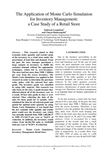
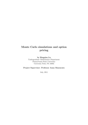
0.1Introduction to Monte Carlo SimulaionMonte Carlo Option Price is a method often used in Mathematical finance to calculate the value of an option with multiple sources of uncertainties and random features, such as changing interest rates, stock prices orexchange rates, etc. This method is called Monte Carlo simulation, namingafter the city of Monte Carlo, which is noted for its casinos. In my project, Iuse Mathematica, a mathematics computer software, we can easily createa sequence of random number indicating the uncertainties that we mighthave for the stock prices for example.0.2Pricing Financial Options by Flipping a CoinA distcrete model for change in price of a stock over a time interval [0,T] is Sn 1 Sn µSn t σSn εn 1 t,S0 s(1)where Sn Stn is the stock price at time tn n t, n 0, 1, ., N 1, t T /N , µ is the annual growth rate of the stock, and σ is a measure of thestocks annual price volatility or tendency to fluctuate. Highly volatile stockshave large values of σ. Each term in sequence ε1 , ε2 . takes on the valueof 1 or -1 depending on the outcoming value of a coin tossing experiment,heads or tails respectively. In other words, for each n 1,2,.(1 with probability 1/2εn (2) 1 with probability 1/2By using Mathematica, it is very easy to create a sequence of random number. With this sequence, the equation (1) can then be used to simulatea sample path or trajectory of stock prices, {s, S1 , S2 , ., SN }. For ourpurpose here, it has been shown as a relatively accurate method of pricingoptions and very useful for options that depend on paths.0.30.3.1Proof of highly volatile stocks have large values for σσ 0.01Let us simulate several sample trajectories of (1) for the following parametervalues and plot the trajectoris: µ 0.12, σ 0.01, T 1, s 40, N 254.The following figures are the graphs that we got for σ 0.01 Since wehave ε to be the value generated by flipping a coin, it gives us arbitrary valuesand thus, we have different graphs for parameter σ 0.01, µ 0.12, T 1, s 40, N 254This is another possibile graph.1

Figure 1: Let M be the value of S254 of different trajectories, k is the numberof trajectories0.3.2σ 0.7Then we repeated the experiment using the value of σ 0.7 for the volalityand other parameters remain the same.Similarly, it should have a number of different graphs due to the arbitraryvalue of ε we generated by Mathematica. The following figures are thegraphs that we got for σ 0.7Conclusion: From the two experiments above with the large differentσ and constant other parameters, we can tell that the larger the σ, thegreater degree of variability in their behavior forthe ε ’s it is permissibleto use random number generator that creates normally distributed randomnumbers with mean zero and variance one. Recall that the standard normaldistribution has the bell-shape with a standard deviation of 1.0 and standardnormal random variable has a mean of zero.0.4Monte Carlo Method vs. Black-Scholes Model0.4.1Monte Carlo Method and its computingMonte Carlo Method In the formular (1), the random terms Sn εn 1 t on the right-hand sidecan be consider as shocks or distrubances that model functuations in thestock price. After repeatedly simulating stock price trajectories, as we didin the previous chapter, and computing appropriate averages, it is possibleto obtain estimates of the price of a European call option, a type of2

45444342410.20.40.60.81.0Figure 2: S254 45.415, σ 0.01financial derivative. A statistical simulation algorithm of this type is whatwe known as ”Monte Carlo method”A European call option is a contract between two parties, a holder and awriter, whereby, for a premium paid to the writer, the holder can purchasethe stock at a future date T (the expiration date) at a price K (the strikeprice) agreed upon in the contract. If the buyer elect to exercise the optionon the expiration date, the writer is obligated to sell the inderlying stockto the buyer at the price K, the strike price. Thus, the option has a payofffunctionf (S) max(S K, 0)(3)where S S(T ) is the price of the underlying stock at the time T whenthe option expires. This equation (3) produces one possible option value atexpiration and after computing this thousands of times in order to obtain afeel for the possible error in estimating the price. Equation(3) is also knownas the value of the option at time T since if S(T ) K, the holder can purchase, at price K, stock with market value S(T) and thereby make a profitequal toS(T ) K not counting the option premium. However, on the otherhand, if S(T ) K, the holder will simply let the option expire since therewould be no reason to purchase stock at a price that exceeds the marketvalue.In other words, the option valuation problem is determine the correctand fair price of the option at the time that the holder and writer enterinto the contract. In order to estimate the price call of a call option using aMonte Carlo method, an ensembleno(k)(4)SN S (k) (T ), k 1, .M3

45444342410.20.40.60.81.0Figure 3: S254 45.1316, σ 0.01of M stock orices at expiration is generated using the difference equation (k)(k)(k)S0 s(5)Sn 1 Sn(k) rSn(k) t σSn(k) εn 1 t,Equation (5) is identical to equation (1) for eachk 1, ., M , except thegrowth rate µ is replaces by the annual interest r that it costs the writerto borrow money.Option pricingotheory requires that the average value ofn(k)the payoffs f (SN 0, k 1, ., M be equal to the compounded total returnobtained by investing the option premium, Ĉ(s), at rate r over the life ofoption,M1 X(k)f (sN ) (1 r t)N Ĉ(s).(6)Mk 1Solving(6) for Ĉ(s) yields the Monte Carlo estimate)(MX1(k)f (sN )Ĉ(s) (1 r t) NM(7)k 1for the option price. So, the Monte Carlo estimateĈ(s) is the present valueof the average of the payoffs computed using rules of compound interest.0.4.2Computing Monte Carlo EstimateWe use equation (7) to compute a Monte Carlo estimate of the value of a five5month call option, in other word T 12years, for the following parametervalues: r 0.06, σ 0.2, N 254, andK 50. N is the number of timesof steps for each trajectories.4

45444342410.20.40.60.81.0Figure 4: S254 45.1881, σ 0.010.5Comparing to the Exact Black-Scholes FormularMonte Carlo has been used to price standard European options, but aswe known that Black-Scholes model is the correct method of pricing theseoptions, so it is not necessary to use Monte Carlo simulation.Here is the formular for exact Black-Scholes model: sK d1C(s) erf c( ) e rT erf c(f rac d2 2)(8)222where sσ21d1 [ln( ) (r )T ], d2 d1 σ Tk2σ Tand erfc(x) is the complementary error function,Z 22erf c(x) e t dtπ x(9)(10)Now we insert all data we have to the Black-Schole formula to check theaccuracy of our results by comparing the Monte Carlo approximation withthe value computed from exact Black-Schole formula. We generated BlackScholes Model with parameterr 0.06, σ 0.2, K 50, k 1, ., M (whereT N t), N 200. And we got: C(40) 1.01189, C(45) 2.71716 and C(50) 5.49477. The error of the Monte Carlo Estimate seems to be very large.Thus we repeat the previous procedure and increased our sample size (M)to 50,000 and 100,000. Then, I made a chart to check if the accuracy ofMonte Carlo Simulation increases by the increasing of the sample size.5

45444342410.20.40.60.81.0Figure 5: S254 45.5859, σ 0.01Comparison of the accuracy of the Monte Carlo Estimate to the BlackSchole ModelMCE(1,000)Ĉ(40) 1.67263Ĉ(45) 4.6343Ĉ(50) 8.1409MCE (10,000)Ĉ(40) 1.61767Ĉ(45) 4.24609Ĉ(50) 7.92441MCE (50,000)Ĉ(40) 1.76289Ĉ(45) 4.3014Ĉ(50) 7.7889MCE (100,000)Ĉ(40) 1.7496Ĉ(45) 4.2097Ĉ(50) 7.6864Black-Schole ModelBS(40) 1.71179BS(45) 4.11716BS(50) 7.49477By the comparing Monte Carlo Estimate and the Black-Schole modle, wecan tell quite easily that the error gets smaller as the sample size increases.Here we calculated the relative error by the equationM onteCarloEstimate Black ScholemodleBlack ScholeM odle(11)The results areerror(1,000)E(40) 0.60593E(45) 0.32330E(50) 0.24272error (10,000)E(40) 0.30232E(45) 0.19466E(50) 0.07819error(50,000)E(40) 0.14037E(45) 0.13862E(50) 0.05254error (100,000)E(40) 0.14037E(45) 0.08833E(50) 0.02157Conclusion: Monte Carlo Simulation gives the option price is a sampleaverage, thus according to the most elementary principle of statistics, itsstandard deviation is the standard deviation of the sample divided by thesquare root of the sample size. So, the error reduces at the rate of 1 overthe square root of the sample size. To sum up, the accuracy of Monte CarloSimulation is increasing by increasing the size of the sample.6Black-Schole ModelBS(40) 1.71179BS(45) 4.11716BS(50) 7.49477

Figure 6: replaced previous value of sigma with 0.70.6Comparing to the Variance Reduction by Antitheric VariattesVariance Reduction by Antithetic Variates is a simple and morewidely used way to increase the accuracy of the Monte Carlo Simulation. Itis the technique used in some certain situations with an additional increasein computational complexity is the method of antithetic variates. In orderto achieve greater accuracy, one method of doing so is simple and automatically doubles the sample size with only a minimum increase in computationaltime. This is called the antithetic variate method. Because we are generating obervations of a standard normal random variable which is distributedwith a mean of zero, a variance of 1.0 and symmetric, there is an equallylikely chance of having drawn the observed value times 1. Thus, for eacharbitrary ε we draw, there should be an artificially observed companion observation of ε that can be legitimately created by us. This is the antitheticvariate.For each k 1,.,M use the sequenceno(k)(k)ε1 , ., εN 1(12)no(k)(k)k 1in equation (5) to simulate a payoff f (SN)and also use the sequence ε1 , ., εN 1k in equation (5) to simulatean associatedno payoff f (SN ). Now the payoffsk k are simulated inpairs f (SN), f (SN) This is the Mathematica Programthat we ran to evaluate the Variance Reduction.After comparing Monte Carlo Simulation with Variance Reduction byAntithetic Variates, We made a table of data.7