Transcription
Applied Mathematics, 2014, 5, 1152-1168Published Online May 2014 in SciRes. 0.4236/am.2014.58108The Application of Time Series Modellingand Monte Carlo Simulation: ForecastingVolatile Inventory RequirementsRobert Davies, Tim Coole, David OsipywFaculty of Design Media and Management, Buckinghamshire New University, High Wycombe, UKEmail: rdavie01@bucks.ac.ukReceived 8 January 2014; revised 8 February 2014; accepted 15 February 2014Copyright 2014 by authors and Scientific Research Publishing Inc.This work is licensed under the Creative Commons Attribution International License (CC tractDuring the assembly of internal combustion engines, the specific size of crankshaft shell bearing isnot known until the crankshaft is fitted to the engine block. Though the build requirements for theengine are consistent, the consumption profile of the different size shell bearings can follow ahighly volatile trajectory due to minor variation in the dimensions of the crankshaft and engineblock. The paper assesses the suitability of time series models including ARIMA and exponentialsmoothing as an appropriate method to forecast future requirements. Additionally, a Monte Carlomethod is applied through building a VBA simulation tool in Microsoft Excel and comparing theoutput to the time series forecasts.KeywordsForecasting, Time Series Analysis, Monte Carlo Simulation1. IntroductionInventory control is an essential element within the discipline of operations management and serves to ensuresufficient parts and raw materials are available for immediate production needs while minimising the overallstock holding at the point of production and throughout the supply chain. Methodologies including MaterialsRequirements Planning and Just-in-Time Manufacturing have evolved to manage the complexities of supplymanagement supported by an extensive academic literature. Similarly extensive study into the inventory profilesfor spare part and service demand has also been prevalent over the last 50 years.This paper presents a study of an inventory process that does not fit into the standard inventory models withinconventional operations management or for service and spare parts management. In high volume internal comHow to cite this paper: Davies, R., et al. (2014) The Application of Time Series Modelling and Monte Carlo Simulation:Forecasting Volatile Inventory Requirements. Applied Mathematics, 5, 1152-1168.http://dx.doi.org/10.4236/am.2014.58108
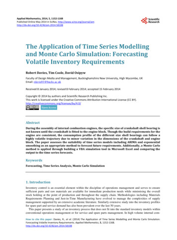
R. Davies et al.bustion engine manufacturing, the demand profile for crankshaft shell bearings follows a highly variable demandprofile though there is consistent demand for the engines. The paper reviews the application of both time seriesanalysis and a Monte Carlo simulation method to construct a robust forecast for the shell usage consumption.Section 2 presents the problem statement. Time series analysis is reviewed in Section 3. The Monte Carlo simulation method written in Microsoft Excel VBA is presented in Section 4. Forecasts generated by both the timeseries models and the simulation are assessed in Section 5 and concluding remarks are presented in Section 6.The analysis utilises usage data provided by a volume engine manufacturer over a 109-week production buildperiod.2. Problem StatementThe construction of petrol and diesel engines involve fitting a crankshaft into an engine block and attaching piston connecting rods to the crankshaft crank pins [1]. The pistons via the connecting rods turn the crankshaftduring the power stroke of the engine cycle to impart motion. Shell bearings are fitted between the crank journals and crank pins and the engine block and connecting rods. During engine operation a thin film of oil underpressure separates the bearing surface from the crankshaft journals and pins. For the smooth operation of the engine, the thickness of the oil film has to be consistent for each crank journal and pin. Though the crankshaft,connecting rods and engine block are machined to exceptionally tight tolerances minor deviations in the dimensions of the machined surfaces mean that the thickness of the oil film will not be consistent across the individualcrank journals and pins.To overcome the problem, the engine designer specifies a range of tolerance bands within an overall tolerancefor the nominal thickness of the shell bearing. Similar tolerance bands are specified for the machined surfaces ofthe engine block and crankshaft. A shell bearing whose thickness is defined within a specific tolerance band isidentified by a small colour mark applied during the shell manufacturing process. The engine designer creates a“Fitting Matrix”, where the combination of the tolerance bands for the engine block and crankshaft are compared against which the appropriate shell bearing can be selected. During the engine assembly, the selectionprocess is automated. Embossed marks on the crankshaft and engine block specify the tolerance bands of eachmachined surface. The marks are either optically scanned or fed into a device that creates a visual display of thecolours of the shells to select for assembly. Selection is rapid and does not impede the speed of engine assembly.Table 1 illustrates the set of tolerance bands and associated “Fitting Matrix” for the selection of main bearingshells for a typical engine.Over time the usage profile for some shells thicknesses can show considerable variation against a consistentdemand for the engine itself. The high variation poses a difficult procurement problem for engine assemblersthat support high volume automotive production. It is difficult to determine what the usage consumption for highusage shells will be over a future time horizon as the shell bearings can be globally sourced and can require leadtimes of between 3 and 6 months.Figure 1 illustrates the consumption trajectory of journal shell sizes over a 109-week sample period that hashigh demand profiles. The shells are identified by the colour green and yellow. The green shell consumption ishighly volatile with sporadic spikes in demand. The yellow shell consumption after showing a rapid decline overFigure 1. Time series trajectories for green and yellow shell consumption.1153
R. Davies et al.Table 1. Bearing selection-fitting matrix.Dimension TableEngine Block: Main BearingUpp TolDia 59 mmLwr TolCrankshaft Main Bearing 0.024 μm 0 μmUpp Tol 0.008 μmLwr Tol 0.016 μmDia 55 mmRange (μm)MarkMain BearingThickness 2 mmRange (μm)MarkUpp Tol 0.012 μmLwr Tol 0.06 μmRange (μm)ColourA0 61 8 4Blue 12 9B 6 122 40Black 9 6C 12 1830 4Brown 6 3D 18 244 4 8Green 305 8 12Yellow0 36 12 16Pink 3 6Fitting MatrixMain lack/Blue6BrownBlackBlack/BlueBlueEngine Blockthe first 30 weeks of the sample period settles to lower and less volatile demand than the green shell.3. Time Series AnalysisSuccinctly, a time series is a record of the observed values of a process or phenomena taken sequentially overtime. The observed values are random in nature rather than deterministic where the random behaviour is moresuitable to model through the laws of probability. Systems or processes that are non-deterministic in nature arereferred to as stochastic where the observed values are modelled as a sequence of random variables. Formally:A stochastic process {Y ( t ) ; t T } is a collection of random variables where T is an index set for which allthe random variables Y ( t ) , t T , are defined on the same sample space. When the index set T represents time,the stochastic process is referred to as a time series [2].While time series analysis has extensive application, the purpose of the analysis is two-fold [3]. Firstly to understand or model the random (stochastic) mechanism that gives rise to an observed series and secondly to predict or forecast the future values of a series based on the history of that series and, possibly, other related seriesor factors.Time series are generally classified as either stationary or non stationary. Simplistically, stationary time seriesprocess exhibit invariant properties over time with respect to the mean and variance of the series. Conversely,for non stationary time series the mean, variance or both will change over the trajectory of the time series. Stationary time series have the advantage of representation by analytical models against which forecasts can beproduced. Non stationary models through a process of differencing can be reduced to a stationary time seriesand are so open to analysis applied to stationary processes [4].1154
R. Davies et al.An additional method of time series analysis is provided by smoothing the series. Smoothing methods estimate the underlying process signal through creating a smoothed value that is the average of the current plus pastobservations.3.1. Analysis of Stationary and Non-Stationary Time SeriesStationary time series are classified as having time invariant properties over the trajectory of the time series. It isthese time invariant properties that are stationary while the time series itself appears to fluctuating in a randommanner. Formally, an observed time series {Y ( t ) ; t T } is weakly stationary if the following properties hold:1) E Y ( t ) µ , t T σ 2 2) Var Y ( t ) ()3) Cov Yt , Yt j γ j , t , j TFurther, the time series is defined as strictly stationary if in addition to Properties 1-3, if subsequently:4) The joint distribution of {Y ( t1 ) , Y ( t2 ) , , Y ( tk )} is identical to {Y ( t1 h ) , Y ( t2 h ) , , Y ( tk h )} forany ti , h T .Conversely, a non-stationary time series will fail to meet either or both the conditions of Properties 1 and 2.Property 3 states that the covariance of lagged values of the time series is dependent on the lag and not time.Subsequently the autocorrelation coefficient ρ k at lag k is also time invariant and is given by ρkCov ( yt , yt k ) γ k γ0Var ( yt )(1)The set of all ρ k , k 0,1, 2, , n forms the Autocorrelation Function or ACF. The ACF is presented as agraphical plot. Figure 2 provides an example of a stationary time series with the associated ACF diagram. Successive observations of a stationary time series should show little or no correlation and is reflected in the ACFplot showing a rapid decline to zero.Conversely, the ACF of a non stationary process will show a gentler decline to zero. Figure 3 replicates theACF for a non-stationary random walk process.Stationary time series models are well defined throughout the time series literature where a full treatment oftheir structure can be found. Representative references include [5]-[8].A consistent view of a time series is that of a process consisting of two components a signal and noise. Thesignal is effectively a pattern generated by the dynamics of the underlying process generating the time series.The noise is anything that perturbs the signal away from its true trajectory [7]. If the noise results in a time seriesthat consists of uncorrelated observations with a constant variance, the time series is defined as a white noiseprocess. Stationary time models are always white noise processes where the noise is represented by a sequenceof error or shock terms {ε t } where ε t N ( 0, σ ) . The time series models applicable to stationary and non stationary time series are listed in Table 2.From Table 2, it is seen that by setting the p, d, and q parameters to zero as appropriate, the MA(q), AR(p)and ARMA(p, q) processes can be presented as sub processes of the ARIMA(p, d, q) process and is illustrated inthe hierarchy presented in Figure 4. The stationary processes can be thought of as ARIMA processes that do notrequire differencing.Table 2. Description of time series models.1) Moving Average Process MA(q): The time series yt is defined as the sum of the process mean and the current shock value plus aweighted sum of the previous “q” past shock values.2) Autoregressive Process AR(p): The time series yt is presented as a linear dependence of weighted “p” observed past values summedwith the current shock value and a constant.3) Autoregressive Moving Average ARMA(p, q): The time series yt is presented as a mixture of both moving average and autoregressiveterms. ARMA(p, q) processes require fewer parameters when compared to the AR or MA process (Chatfield, 2006).4) Autoregressive Integrated Moving Average ARIMA (p, d, q): A non stationary time series is transformed into a stationary time seriesthrough a process of differencing. The ARIMA process differences a time series at most d times to obtain a stationary ARMA(p, q) process.1155
R. Davies et al.Figure 2. Stationary time series—example ACF.Figure 3. Non-stationary time series example ACF (Random walk).Figure 4. Time series model hierarchy.Moreover, the ARIMA process reveals time series models that are not open to analysis by the stationary representations. Two such models are included in Figure 4, the random walk model, ARIMA(0, 1, 0) and the exponential moving average model, ARIMA(0, 1, 1).Table 3 returns the modelling processes that are applied to stationary and non-stationary time series. The1156
R. Davies et al.Table 3. Synthesis of time series models.ProcessMA(q)AR(p)Modelyt µ ε t θ1ε t 1 θ 2ε t 2 θ qε t qyt µ Θ ( B ) ε tyt δ φ1 yt 1 φ2 yt 2 φ p yt p ε tΦ ( B ) yt δ εtpARMA(p, q)Stationary ConditionNone: MA(q) process is always stationary.p φi 1i 1qyt δ φi yt i ε t θiε t i i 1 i 1AR(p) component is stationary.Φ ( B ) yt δ Θ ( B ) ε tARIMA(p, d, q)Φ ( B )(1 B ) yt δ Θ ( B ) ε tdThe AR(p) component is stationary after the series isdifferenced d times.equations of the models are replicated in their standard form and in terms of the backshift operator B (see Appendix 1). Time series models expressed in terms of the backshift operator are more compact and enable a representation for the ARIMA process that has no standard form equivalent.3.2. Model IdentificationInitially, inspection of the ACF of a time series is necessary to determine if the series is stationary or will requiredifferencing. There is no analytical method to determine the order of differencing though empirical evidencesuggests that generally first order differencing (d 1) is sufficient and occasionally second order differencing (d 2) should be enough to achieve a stationary series [7].The ACF is also useful to indicate the order of the MA(q) process as it can be shown that for k q , ρ k 0 .Hence the ACF will cut off at lag q for the MA(q) process. The ACF of the AR(p) and ARMA(p, q) processesboth exhibit exponential decay and damped sinusoidal patterns. As the form of the ACF’s for these processes isindistinguishable, identification of the process is provided by the Partial Autocorrelation Coefficient (PACF).The properties of the PACF are discussed extensively in the time series literature and in particular a comprehensive review provided in [9]. Descriptively, the PACF quantifies the correlation between two variables that isnot explained by their mutual correlations to other variables of interest. In an autoregressive process, each termis dependent on a linear combination of the preceding terms. In evaluating the autocorrelation coefficient ρ k ,the term yt is correlated to yt k . However, yt is dependent on yt 1 which in turn is dependent on yt 2 and thedependency propagates throughout the time series to yt k . Consequently, the correlation at the initial lag of thetime series propagates throughout the series. The PACF evaluates the correlation between xt is and xt kthrough removing the propagation effect.The PACF can be calculated for any stationary time series. For an AR(p) process, it can be shown that thePACF cuts off at lag p. The PACF for both the MA(q) and ARMA(p, q) process the PACF is a combination ofdamped sinusoidal and exponential decay.The structure of a stationary time series is determined through inspection of both the ACF and PACF diagrams of the series. Table 4 presents the classification of the stationary time behaviour (adapted from [7] [8]).Neither the ACF nor PACF yield any useful information with respect to identifying the order of the ARMA (p,q) process. Though there are additional methods that can aid the identification of the required order of theprocess [7] [8] including the extended sample autocorrelation function (ESACF), the generalised sample partialautocorrelation function (GPACF), and inverse autocorrelation function (IACF) as suitable methods for determining the order of the ARMA model. However, with respect to investigating the structure of a time series bothsets of authors agree that with the availability of statistical software packages it is easier to investigate a range ofmodels with various orders to identify the appropriate model and forego the need to apply these additional methods.The estimation of the parameter coefficients φi and θi can be estimated through Maximum Likelihood Estimation (MLE). An extensive explanation of the MLE application to estimate the parameters of each the models1157
R. Davies et al.Table 4. Classification of stationary time series behavior.ModelACFPACFMA(q)Cuts off after lag qInfinite exponential decay and/or dampedsinusoid—tailing offAR(p)Infinite exponential decay and/or dampedsinusoid—tailing offFinite-cuts off after lag pARMA(p,q)Infinite exponential decay and/or dampedsinusoid—tailing offInfinite exponential decay and/or dampedsinusoid—tailing offlisted in Table 2 is provided in [10]. Additionally the parameters of the AR(p) process can be calculated withthe Yule Walker Equations [4] [9].The robustness of a derived model is assessed through residual analysis of the model. For the ARMA(p, q)process the residual are obtained from pq ˆεˆt yt δˆ φˆi yt 1 θεt 1 i 1 i 1 (2)If the residual values exhibit white noise behaviour, the ACF and PACF diagrams of the residual valuesshould not show any discernable pattern then the appropriate model has been chosen and the correct orders of pand q have been correctly identified.3.3. Generation of ForecastsEstablishing a model that describes the structure of an observed time series enables meaningful forecasts to bedrawn from the model. Forecasting methods for each of the models in Table 2 are succinctly described in [11]and are defined as follows:AR(p) Process:The forecast for the AR(p) process is based on the property that the expectation of the error terms ε i arezero. The forecast is developed iteratively from the previous observation to create a one step ahead forecast. Thestep ahead is denoted byτ 1: yˆt (1) δ φ1 yt 1 φ2 yt 2 φ p yt p 1τ 2 : yˆt ( 2 ) δ φ1 yˆt (1) φ2 yt 2 φ p yt p 2At each successive iteration, the most recent observation drops out of the forecast and replaced by the previous forecast value. At τ p , each term is a forecasted value and continuing the iteration process, the forecastconverges onto the mean of the AR(p) process.MA(q) Process:The expectation of the ε i terms in the MA(q) process follow a white noise process and so the expectation ofall future values of ε i , i 0 is zero. Hence for t q the forecast of a MA(q) process is just the mean value ofthe process, µ .ARMA(p, q) Process:The forecast for the ARMA(p, q) process is the combination of the results from the pure AR(p) and MA(q)processes. For t q, the error terms completely drop out of the forecast.3.4. Smoothing MethodsSmoothing methods provide a class of time series models that have the effect of reducing the random variationof a time series with the effect of exposing the process signal within the time series. A variety of smoothingmodels that average the series continually over a moving span of observed values or fit a polyn
method is applied through building a VBA simulation tool in Microsoft Excel and comparing the output to the time series forecasts. Keywords Forecasting, Time Series Analysis, Monte Carlo Simulation 1. Introduction Inventory control is an essential element within the discipline of operations management and serves to ensure