WIXLIB

2.2Sample StatisticsTo be able to use the statistical measures defined above, we need ways to estimatethe statistics using measured data. Here, we give the sample statistics, which areunbiased estimators of the above measures in the sense that they approach the truevalues of the measures as the number of measurements increases.Let us consider a n p matrix of data, where each column contains n measurements for variables x1 , ., xp : x1x11 x21 X . .xn1x2x12x22.xp x1px2p . . xn2. . . xnp(9)In this course, we need the following sample statistics: the sample mean for the kth variable isx̂k n1Xxikn i 1(10) the sample variance of the kth variable isn1 X(xik x̂k )2 σk2Var(xk ) n 1 i 1(11) the sample standard deviation isStd(xk ) p(Var(xk )) σk(12) the sample covariance between two variables isn1 XCov(xk , xl ) (xik x̄k )(xil x̄l ) : σxk xln 1 i 1 the sample correlation coefficient between two variables isσ xk xlCor(xk , xl ) : ρxk xlσxk σxl(13)(14)The sample variances and covariances for p variables can be compactly representedas a sample covariance matrix, which is given as 2σσx1 x2 . . . σx1 xp x1 σx1 x2 σx22 .Cov(X) (15) . . σx1 xpσx2p7

That is, the variances of the variables are given in the diagonal of the covariancematrix, and the off-diagonal elements give the individual covariances. Similarly, onecan form a correlation matrix using the relationship of covariance and correlationgiven in equation (14), with ones in the diagonal and correlation coefficients betweenthe variables in the off-diagonal: 1ρx1 x2 . . . ρx1 xp ρx1 x2 1 .Cor(X) .(16) . . ρx1 xp1Note that here we use partly the same notation for the definition of the statisticalmeasures and their corresponding sample statistics. In the rest of the course, we willonly need the sample statistics, and in what follows, Var means sample variance,Cov means sample covariance matrix and so on.2.3Some distributionsIn this course, we need some basic distributions. The distribution of a randomvariable x is characterized by its probability density function (PDF) p(x).The PDF of the univariate normal (or Gaussian) distribution with mean x0 andvariance σ 2 is given by the formula 2 !1 x x01exp .(17)p(x) 2σ2πσ2For a random variable x that follows the normal distribution, we writePn x 2 N(x0 , σ ).Let us consider a sum of n univariate random variables, s i 1 xi . The sumfollows the chi-square distribution with n degrees of freedom, which we denote bys χ2n . The density function for the chi-square distribution isp(s) 1/(2n/2 Γ(n/2))sn/2 1 e s/2 .(18)The most important distribution in this course is the multivariate normal distribution. The d-dimensional Gaussian distribution is characterized by the d 1 meanvector x0 and the d d covariance matrix Σ. The probability density function is 11T 1p(x) exp (x x0 ) Σ (x x0 ) ,(19)(2π)d/2 Σ 1/22where Σ denotes the determinant of Σ.Let us consider a zero-mean multivariate Gaussian with covariance matrix Σ.The term in the exponential can be written as xT Σ 1 x yT y, where y Σ 1/2 x.Here Σ1/2 and Σ 1/2 denote the ’square roots’ (e.g. Cholesky decompositions) ofthe covariance matrix and its inverse, respectively. Using the formula for computing8

the covariance matrix of a linearly transformed variable, see equation (22) in thenext section, the covariance of the transformed variable can be written ascov(Σ 1/2 x) Σ 1/2 cov(x)(Σ 1/2 )T Σ 1/2 Σ(Σ 1/2 )T Σ 1/2 Σ1/2 (Σ1/2 Σ 1/2 )T I,(20)T 1Twhere I is the identity matrix. That is, the term x Σ x y y is a squared sumof d independent standard normal variables, and therefore follows the chi-squaredistribution with d degrees of freedom:xT Σ 1 x χ2d .(21)This gives us a way to check how well a sampled set of vectors follows a Gaussiandistribution with a known covariance matrix: compute the values xT Σ 1 x for eachsample and see how well the statistics of the values follow the χ2d distribution (seeexercises).The contours of multivariate Gaussian densities are ellipsoids, where the principal axes are given by the eigenvectors of the covariance matrix, and the eigenvaluescorrespond to the lengths of the axes. Therefore, two-dimensional covariance matrices can be visualized as ellipses. In practice, this can be done with the ellipsefunction given in the code package, see help ellipse. In Fig. 2.3 below, ellipsescorresponding to three different covariance matrices are illustrated (the figure isproduced by the program ellipse Figure 1: Ellipses corresponding to the 90% confidence region for three covariancematrices, diagonal (left), with correlation 0.9 (center) and with correlation 0.7(right).2.4Generating Gaussian random numbersLater in the course, we need to be able to generate random numbers from multivariate Gaussian distributions. A basic strategy is given here. Recall that in theunivariate case, normal random numbers y N (µ, σ 2 ) are generated by y µ σz,where z N (0, 1).It can be shown (see exercises) that the covariance matrix of a random variablemultiplied by a matrix A iscov(Ax) Acov(x)AT .9(22)

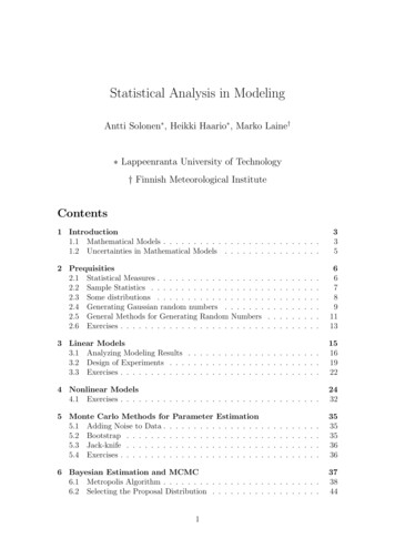
This is a useful formula when random variables are manipulated. For instance, letus consider a covariance matrix Σ, which we can decompose into a ’square-root’form Σ AAT . Now, if we take a random variable with cov(x) I, the covariancematrix of the transformed variable Ax iscov(Ax) Acov(x)AT AAT Σ.(23)This gives us a recipe for generating Gaussian random variables with a given covariance matrix:ALGORITHM: generating zero mean Gaussian random variables y withcovariance matrix Σ1. Generate standard normal random numbers x N(0, I).2. Compute decomposition Σ AAT .3. Transform the standard normal numbers with y Ax.In practice, the standard normal random numbers in step 1 can be generated usingexisting routines built in to programming environments (in MATLAB using therandn command). The matrix square root needed in step 2 can be computed,for instance, using the Cholesky decomposition (the chol function in MATLAB).However, note that any symmetric decomposition Σ AAT will do. Note thatthe approach is analogical to the one-dimensional case, where standard normalnumbers are multiplied with the square root of the variance (standard deviation).Non-zero Gaussian variables can simply be created by adding the mean vector to thegenerated samples. Generating multivariate normal random vectors is demonstratedin the program randn demo.mGaussian random number generation has also an intuitive geometric interpretation. If the covariance matrix can be written as a sum of outer products of nvectors (a1 , ., an ),nXΣ ai aTi ,(24)i 1it is easy to verify that the sumy nXωi ai ,(25)i 1where ωi are standard normal scalars, ωi N (0, 1), follows the Gaussian distribution with covariance matrix Σ. That is, Gaussian random variables can be viewedas randomly weighted combinations of ’basis vectors’ (a1 , ., an ). This interpretation is illustrated for a two-dimensional case in Fig. 2.4. For an animation, see alsothe demo program mvnrnd demo.m.10

re 2: Black lines: two vectors a1 andPa2 and the 95% confidence ellipse correTsponding to the covariance matrix Σ 2i 1 ai aPi . Green lines: weighted vectorsω1 a1 and ω2 a2 . Red dot: one sampled point y 2i 1 ωi ai .2.5General Methods for Generating Random NumbersIn this section, we consider two methods to sample from non-standard distributions,whose density function is known: the inverse CDF technique and the accept-rejectmethod. Another important class of random sampling methods, the Markov chainMonte Carlo (MCMC) methods, is covered separately in Section 6.Inverse CDF MethodLet us consider a continuous random variable whose cumulative distribution function (CDF) is F . The inverse CDF method is based on the fact that a randomvariable x F 1 (u) where u is sampled from U [0, 1], and F 1 is the inverse function of F , has the distribution with CDF F . The inverse CDF method can bevisualized so that uniform random numbers are ’shot’ from the y-axis to the CDFcurve and the corresponding points in the x-axis are samples from the correct target,as illustrated for the exponential distribution in Fig. 2.5.The inverse CDF method is applicable, if the cumulative distribution functionis invertible. For distributions with non-invertible CDF, other methods need to beapplied. If one has a lot of samples, one can approximate the CDF of the distributionby computing the empirical CDF function, and generate random variables usingthat. In addition, the inverse CDF method is a good way to draw samples fromdiscrete distributions, where the CDF is essentially a step function.11

gure 3: Producing samples from the exponential distribution using inverse CDF,F (x) 1 exp( x) and F 1 (u) ln(1 u).Accept-Reject MethodSuppose that f is a positive (but non-normalized) function on the interval [a, b],bounded by M. If we generate a uniform sample of points (xi , ui ) on the box [a, b] [0, M ], the points that satisfy ui f (xi ) form a uniform sample under the graph off.The area of any slice {(x, y) xl x xu , y f (x)} is proportional to thenumber of sampled points in it. So the (normalized) histogram of the points xigives an approximation of the (normalized) PDF given by f . The accept-rejectmethod is illustrated in Fig. 2.5The method is not restricted to 1D, the interval [a, b] may have any dimension.We arrive at the following algorithm: Sample x U ([a, b]), u U ([0, M ]). Accept points x for which u f (x)So, we have a (very!) straightforward method that, in principle, solves ’all’sampling problems. However, difficulties arise in practice: how to choose M andthe interval [a, b]. M must be larger that the maximum of f , but too large a valueleads to many rejected samples. The interval [a, b] should contain the support of f– which generally is unknown. A too large interval again leads to many rejections.Moreover, uniform sampling in a high dimensional interval is inefficient in any case,if the support of f only is a small subset of it.12

re 4: Left: In accept-reject, points are sampled in the box [a, b] [0, M ] (greenline), and points that fall below the target density function (blue line) are accepted(black points) and the other points are rejected (red points). Right: the histogramof the sampled points.2.6Exercises1. Generate random numbers from N(µ, σ 2 ) with µ 10 and σ 3. Study howthe accuracy of the empirical mean and standard deviation behaves as thesample size increases.2. Generate samples from the χ2n distribution with n 2 and n 20 in threedifferent ways:(a) by the definition (computing sums of normal random numbers)(b) by the inverse CDF method (e.g. using the chi2inv MATLAB function)(c) directly by the chi2rnd MATLAB functionFor each case, create an empirical density function (normalized histogram)and compare it with the true density function (obtained e.g. by the chi2pdfMATLAB function).3. Generate random samples from a zero-centered Gaussian distribution withcovariance matrix 2 5 .C 5 16Verify by simulation that approximately a correct amount of the sampledpoints are inside the 95% and 99% confidence regions, given by the limits ofthe χ2 distribution (use the chi2inv function in MATLAB). Visualize thesamples and the confidence regions as ellipses (use the ellipse function).4. Show that equation (22) holds.13

5. Using the Accept–Reject method, generate samples from the (non-normalized)density2f (x) e x /2 (sin(6x)2 3 cos(x)2 sin(4x)2 1)As the dominating density, use a) uniform distributions x U ( 5, 5) andu U (0, M ) with suitable M b) the density of the N (0, 1) distribution.14

3Linear ModelsLet us consider a linear model with p variables, f (x, θ) θ0 θ1 x1 θ2 x2 . . . θp xp .Let us assume that we have noisy measurements y (y1 , y2 , ., yn ) obtained atpoints xi (x1i , x2i , ., xni ) where i 1, ., p. Now, we can write the model inmatrix notation:y Xθ ε,(26)where X is the design matrix that contains the measured values for the controlvariables, augmented with a column of ones to account for the intercept term θ0 : 1 x11 x12 . . . x1p 1 x21 x22 . . . x2p X . .(27). . . . . . . 1 xn1 xn2 . . . xnpFor linear models, we can derive a direct formula for the LSQ estimator. It can beshown (see exercises), that the LSQ estimate, that minimizes SS(θ) y Xθ 22 ,is obtained as the solution to the normal equations XT Xθ XT y:θ̂ (XT X) 1 XT y.(28)In practice, it is often numerically easier to solve the system of normal equationsthan to explicitly compute the matrix inverse (XT X) 1 . In MATLAB, one can usethe ’backslash’ shortcut to obtain the LSQ estimate, theta X\y, check out the codeexample given later in this section.To obtain the statistics for the estimate, we can compute the covariance matrixCov(θ̂). Let us make the common assumption that we have independent and identically distributed measurement noise with measurement error variance σ 2 . Thatis, we can write the covariance matrix for the measurement as Cov(y) σ 2 I, whereI is the identity matrix. Then, we can show (see exercises) thatCov(θ̂) σ 2 (XT X) 1 .(29)The diagonal elements of the covariance matrix give the variances of the estimatedparameters, which are often reported by different statistical analysis tools.Let us further assume that the measurement errors are Gaussian. Then, wecan also conclude that the distribution of θ̂ is Gaussian, since θ̂ is simply a lineartransformation of a Gaussian random variable y, see equation (28). That is, theunknown parameter follows the normal distribution with mean and covariance matrix given by the above formulae: θ N(θ̂, σ 2 (XT X) 1 ). That is, the probabilitydensity of the unknown parameter can be written as 1T 1(30)p(θ) K exp (θ θ̂) C (θ θ̂) ,2where K ((2π)d/2 Σ 1/2 ) 1 is the normalization constant and C Cov(θ̂).15

3.1Analyzing Modeling ResultsIn regression models, usually not all possible terms are needed to obtain a good fitbetween the model and the data. In empirical models, selecting the terms used isa problem of its own, and numerous methods have been developed for this modelselection problem.Selecting the relevant terms in the model is especially important for predictionand extrapolation purposes. It can be dangerous to employ a ’too fine’ model. Asa general principle, it is often wise to prefer simpler models and drop terms that donot significantly improve the model performance (A. Einstein: ”a model should beas simple as possible, but not simpler than that”). Too complex models often resultin ’over-fitting’: the additional terms can end up explaining the random noise inthe data. See exercises for an example of the effect of model complexity.A natural criterion for selecting terms in a regression model is to drop termsthat are poorly known (not well identified by the data). When we have fitted alinear model, we can compute the covariance matrix of the unknown parameters.Then, we can compute the ’signal-to-noise’ ratios for the parameters in the model,also known as t-values. For parameter θi , the t-value isti θ̂i /std(θ̂i ),(31)where the standard deviations of the estimates can be read from the diagonal ofthe covariance matrix given in equation (29). The higher the t-value is, the smallerthe relative uncertainty is in the estimate, and the more sure we are that the termis relevant in the model and should be included. We can select terms for which thet-values are clearly separated from zero. As a rule of thumb, we can require that,for instance, ti 3.The t-values give an idea of how significant a parameter is in explaining themeasurements. However, it does not tell much about how good the model fits theobservations in general. A classical way to measure the goodness of the fit is thecoefficient of determination, or R2 value, which is written asP i(y f (xi , b̂))22P i.(32)R 1 (y ȳ)2The intuitive interpretation of the R2 value is the following. Consider the simplestpossible model y θ0 , that is, the data are modeled by just a constant. In thiscase, the LSQ estimate is just the empirical mean of the data, θ̂0 y (see exercises).That is, the R2 value measures how much better the model fits to the data thana constant model. If the model is clearly better than the constant model, the R2value is close to 1.The R2 value tells how good the model fit is. However, it does not tell anythingabout the predictive power of the model, that is, how well the model is able togeneralize to new situations. The predictive power of the model can be assessed,for instance, via cross-validation techniques. Cross-validation, in general, works asfollows:1. Leave out a part of the data from the design matrix X and response y.16

2. Fit the model using the remaining data.3. Using the fitted model, predict the measurements that were left out.4. Repeat steps 1-3 so that each response value in y is predicted.The goodness of the predictions at each iteration can be assessed using the R2formula. The obtained number is called the Q2 value and it describes the predictivepower of the model better than R2 .Cross-validation is commonly used for model selection. The idea is to testdifferent models with different terms included and choose the model that gives thebest Q2 value. If the model is either too complex (’o

The theory for statistical analysis of linear models is well established, and tra-ditionally the linear theory is used as an approximation for nonlinear models as well. However, e cient numerical Monte Carlo techniques, such as Markov Chain Monte Carlo (MCMC), have been introduced lately to allow full