Transcription
Monte Carlo and Binomial Simulations forEuropean Option PricingRobert HonComputer Science with MathematicsSession 2012/2013The candidate confirms that the work submitted is their own and the appropriate credit has beengiven where reference has been made to the work of others.I understand that failure to attribute material which is obtained from another source may beconsidered as plagiarism.(Signature of student)
SummaryThis project looks into how options are priced, exploring different methods and investigating howefficient the approximation techniques are.This project is structured in the following way: Chapter 1 details the aim, objectives, requirementsand methodology of the project. Chapter 2 presents the background research done in the area offinancial modelling, the concept of financial options and how they are price is introduced. Continuedresearch into option pricing led to the famous Black-Scholes model, which is essential for Europeanoptions. In Chapter 3, the Monte Carlo approximation method is implemented and compared to theBlack-Scholes model. Discrete Euler and Milstein schemes are also researched and implemented.The orders of convergence of the implemented methods are analysed. Chapter 4 explores a morecomputationally efficient binomial approximation. This method is compared to the Black-Scholesmodel and in a similar fashion to Chapter 3, the convergence order is analysed. Chapter 5summarises the findings and compares the models to determine which implementationoutperformed other implementations. In Chapter 6, the final conclusions are given and future workpointers are documented.ii
ContentsChapter 1 - Introduction . 11.1 Overview . 11.2 Aim and Objectives . 11.3 Minimum Requirements . 11.4 Methodology. 21.5 Schedule . 3Chapter 2 - Background Research . 42.1 Options . 42.1.1 Call options. 42.1.2 Different Types of Options . 42.2 Asset Price Model . 52.3 Itô’s Lemma. 52.4 The Black-Scholes Model . 62.4.1 Assumptions of the Black Scholes Model . 62.4.2 The Black-Scholes Partial Derivative . 72.4.3 The Black-Scholes Formula for European Options. 82.5 Approximation Techniques . 92.6 Time Discretising Techniques. 9Chapter 3 - Monte Carlo Simulation . 103.1 Monte Carlo Method . 103.1.1 Convergence . 113.2 Time Discretising Methods . 123.2.1 Euler Scheme. 133.2.2 Milstein Scheme . 143.2.3 Convergence . 163.2.4 Runge-Kutta Method . 20iii
Chapter 4 – Binomial Method . 214.1 Valuing the Option . 214.2 Convergence to the Black-Scholes Model. 23Chapter 5 - Evaluation. 255.1 Evaluation of Black-Scholes Model . 255.2 Evaluation of the Monte Carlo Method . 265.3 Evaluation of Euler and Milstein Schemes . 265.4 Evaluation of the Binomial Method . 265.5 Aim and Objectives . 285.6 Minimum Requirements . 29Chapter 6 - Conclusions . 316.1 Future Work . 31Bibliography . 32Appendix A – Personal Reflection . 34Appendix B – External materials used . 36Appendix C – Ethical Issues . 37iv
Chapter 1 - Introduction1.1 OverviewIn a growing option trading financial market, accurate option prices are necessary. There are manydifferent approximation techniques that have been developed through the years. We look into thederivation of these models and analyse which methods are most accurate and computationallyefficient.1.2 Aim and ObjectivesThe aim of this project is to explore option pricing approximation techniques and how theapproximations can be adapted to improve the accuracy.The objectives of the project are to:1) Research into how options are priced.2) Understand the Black-Scholes equation and adapt it to model price European options.3) Implement a Monte Carlo simulation of the European option.4) Explore different time stepping methods, such as the Euler and Milstein schemes, toimprove the accuracy of the approximation.5) Implement the binomial model to approximate the European option.6) Evaluate the accuracy of the implemented models and apply them to American and Asianoptions.1.3 Minimum Requirements1) Produce a Black-Scholes model simulation of the European option.2) Produce a Monte Carlo approximation of the European option.3) Produce a Monte Carlo approximation of the European option using the Euler time steppingmethod.4) Produce a Monte Carlo approximation of the European option using the Milstein timestepping method.5) Produce a binomial approximation of the European option.Possible Extensions:1) Applying refined models to American and Asian options.2) Produce a Monte Carlo approximation of the European option using the Runge-Kutta timestepping method.1
1.4 MethodologyThe first stage of the project is to acquire the underlying theory of option pricing. Therefore researchis conducted around financial options before models can be derived, discretised and simulated. Theresearch explores the different kinds of options and identifies how they are priced differently.Focussing on European options, the derivation and the importance of the Black-Scholes partialdifferential equation from Wilmott et al. (1995) became the fundamental basis. Consequently theBlack-Scholes model is implemented at this stage. The coding was done in Matlab to reduce thelearning overhead of the syntax and GUI of Matlab, as it has been used in COMP2647 NumericalComputation and Visualisation and COMP3920 Parallel Scientific Computing.Research in approximation techniques, from Glasserman (2003) gave a Monte Carlo approachdeveloped by Boyle (1977). Hence the Monte Carlo simulation is implemented and evaluated at thisstage.Glasserman (2003) also gives the basis of discretisation methods, therefore the Euler and Milsteintime stepping method is documented. After understanding the underlying theory the two methodsare then implemented at this stage. The two schemes are evaluated by proving the convergencemeasures documented in Kloeden and Platen (1999).Building on theory from the taught module, MATH3733 Stochastic Financial Modelling, research intothe binomial approximation developed by Cox et al. (1979) is conducted. This method isimplemented and evaluated against the exact value of the European call option from the BlackScholes equation as well as looking at the convergence measure.Finally the binomial model is adapted to implemented American and Asian options based onmethods from Shreve (2005).2
1.5 ScheduleFigure (1.1) The proposed plan at the mid-project report stage.The plan at the mid-project report stage shown in Figure (1.1) was not detailed as there was not aclear direction of the project due to other work commitments. Consequently after the Januaryexamination period, a clear direction of the project was formulated. Therefore the implementationsection was added and the different stages detailed accordingly, the on-going testing and evaluationof different implementations was also added as it is a necessity. The revised Gantt chart is shown inFigure (1.2).Figure (1.2) A revised Gantt chart outlining the schedule of the project.3
Chapter 2 - Background Research2.1 OptionsTo classify what a financial option is, we look at the simplest European call option. It is a contractwith the following conditions and description from Wilmott et al. (1995):At a predetermined timein the future, also known as the time of expiry, the owner of the optionmay purchase the underlying asset for a predetermined price, also known as the exercise price. Theother party of the option is the writer; they have an obligation to sell the asset to the holder if theywant to buy it.In this project we investigate how much the holder should pay for this option, consequently valuingthe option.2.1.1 Call optionsKey notation:, asset price., exercise price., time of expiry in years.Whenat expiry, it would make financial sense to exercise the call option, hence handing overthe amount K, obtaining an asset worth . The profit would be. Ifat expiry, a loss ofwould be made, therefore the option is worthless. The call option can be written as:()()2.1.2 Different Types of OptionsReviewing papers from Broadie and Detemple (2004), Hobson (2004) and Wilmott et al. (1995),below is a brief summary of the most common option styles:Plain Vanilla option types: European options can only be exercised at the time of maturity. American options can be exercised at any time before the time of maturity.Path dependent options: Asian options: The pay-off is calculated from the average price of the asset over a period oftime. Lookback options: The pay-off is dependent on the maximum price reached by the assetover the lifetime of the option.4
Exotic options: Bermudan options can only be exercised a set number of times at certain dates. Barrier options: The option contract can be triggered when the asset price hits apredetermined value at any time before maturity. Digital/Binary options: The pay-off is fixed if the asset crosses the barrier.2.2 Asset Price ModelThe asset price model from Wilmott et al. (1995) states that asset prices must move randomly,therefore: The past history is reflected fully in the current price. The markets immediately respond to new information on an asset.Consequently any unanticipated changes on the asset price are classified as a Markov Process. Asmall time step ofthe assetindicates the change fromto. To model the corresponding return on, we first use , a measure of the average growth rate of the asset, known as the drift.This leads to the termTo model the random element of the asset, the termis used, which is a random variable fromthe normal distribution, also known as a Wiener process.is a measure of the standard deviation ofreturns, also known as the volatility. This leads to the contributionPutting these two results together gives rise to the stochastic differential equationthis equation can be rearranged to give(2.1)2.3 Itô’s LemmaThe following derivation is detailed in 10.2 Hull (1993), B.2 Glasserman (2003), Wilmott et al. (1995)and Kloeden and Platen (1999). Itô’s lemma is a key result that is used to manipulate the randomvariables that are dealt with in this paper.(The call option ( ) is a function of . If is varied by a small amountsmall amount. From the Taylor series expansion,thenwill also vary by acan be written as(5))
the remaining terms, denoted by the dots, is the remainder which is smaller than the other terms wehave retained. Recall Equation (2.1) for,can be calculated by squaring(, hence)()Examining the order of magnitude for the terms in Equation (2.4), (See P29-30 of Wilmott et al.(1995) for order notation). From Equation (2.2) we can see that( )hence the first term of Equation (2.4) dominates the other terms as it is largest for small. Thisleads to the orderSincefrom Equation (2.2), this becomes()By substituting Equation (2.5) into Equation (2.3) and also using the Equation (2.1), we retain termswhich are only as large as ( ), therefore we define Itô’s lemma as()()()2.4 The Black-Scholes ModelThe Black-Scholes model developed by Black and Scholes (1973) is widely accepted to be thestandard way to price European options, the following sections define the key properties of themodel and how it is adapted to price European options.2.4.1 Assumptions of the Black Scholes ModelBlack and Scholes (1973) stated that the following “ideal conditions” are assumed within the market,the stock and the option:1) The interest rate remains constant through time.2) The stock price follows a Geometric Brownian motion where the drift and volatility remainconstant.3) No dividends are paid from the stock.4) The formula is only valid for European options; therefore the option can only be exercised atthe time of maturity.5) No transaction costs are charged when buying or selling.6) Any fraction of the price of a security can be borrowed to buy it or to hold it, at the short6
term interest rate.7) Short selling does not incur any penalties. The seller will accept the price of a security from abuyer if they do not own a security, and agree to settle with the buyer at some future dateby paying him an amount equal to the price of the security on that date.Therefore the Black-Scholes model is a simplified version of the real world model due to theseassumptions.2.4.2 The Black-Scholes Partial DerivativeFrom Wilmott et al. (1995), we can use Itô’s lemma to specify the random walk the value of theoption follows. In this project we are only interested in the call option; hence applying () toItô’s lemma defined in Equation (2.6) gives the random walk followed by()()()Constructing a portfolio consisting of a call option and number of the underlying assetThe difference of the value of the portfolio in one time-interval isApplying Equations (2.1), (2.7) and (2.8) together, we can show that()(follows the random walk)The Black-Scholes model gives an exact solution; hence the random element ofin this randomwalk needs to be eliminated. This is done by substituting()The increment portfolio becomes completely deterministic with this substitution()The assumption of no transaction costs indicates a growth of(in a time interval of)Substituting (2.8) and (2.9) into (2.10) and dividing by, hence(), the resulting equation is the Black-Scholespartial differential equation(An alternative derivation is given in Section 6 of Merton (1973).7)
2.4.3 The Black-Scholes Formula for European OptionsThe following boundary conditions are defined in Wilmott et al. (1995) for European options to findthe unique solution for a European call option.As we are only interested in the call option in this paper, the payoff of the call option is known atfrom Section 2.1.1, hence (time of expiry whenWhen is zero, from Equation (2.1),evolve. Hencetherefore ()()will also be zero, therefore the asset price , can neverat expiry and there is no payoff, consequently the call option is worthless,).If the asset price increases without a limit, the option will be ever more likely to be exercised, themagnitude of the exercise price becomes negligible asas (. Hence the call option can be written)Consequently we put the defined boundary conditions()()()()through Equation (2.11), the partial differential equation. The result gives the following explicitsolution for the European call:(whereand)()()()are denoted as( )() ( ) and() is the cumulative distribution function( ) The detailed derivation of this equation can be found in Chapter 5 of Wilmott et al. (1995), P225-228in Lovelock et al. (2007) and Chapter 7 of Björk (2004).Using Equation (2.12) of the European call, we can compute an option price using this Black-Scholesmodel; therefore a test case is defined. We set the following initial conditions and model parameters: 250, 200, 1, 0.05, 0.2. For the purpose of consistency and validity, these values8
will remain the same in consequent chapters to provide a comparison of results between theimplementation of different models.To calculate the price of the call option, these variables applied to Equation (2.12), to price the calloption. The result is 61.472088609819394.2.5 Approximation Techniques Monte Carlo Method – the derivation and implementation of the Monte Carlo method isdocumented in Section 3.1. Binomial Method – the details of the binomial method is documented and implemented inChapter 4.2.6 Time Discretising Techniques Euler method – the derivation and implementation of the Euler scheme is documented inSection 3.2.1. Milstein Scheme – the derivation and implementation of the Milstein scheme is documentedin Section 3.2.2. Runge-Kutta Methods – the theory of this method is documented in Section 3.2.4.9
Chapter 3 - Monte Carlo Simulation3.1 Monte Carlo MethodRecall that the asset price evolution follows the stochastic differential Equation (2.1). This equationcan be solved to give the Monte Carlo simulation developed by Boyle (1977) to simulate asset paths.( )( )[(( )])()( ) is a random variable, normally distributed with mean 0 and variance T. From Glasserman(2003),( ) can be manipulated to become the distribution , where Z is a standard normalrandom variable with mean 0, and variance 1. Substituting this back into equation (3.1) gives( )( )[() ]To generate the sample paths of the asset, the interval [0,T] is divided into intervals of length[() .]This equation, also stated in Rachev and Ruschendorf (1995) is used to produce Algorithm (3.1) forthe Monte Carlo simulation of a European call option with the initial conditions and modelparameters specified in Section 2.4.3.1 function MonteCarlo {2u ber of p th3u ber of tep4S 250 K 200 r 0.05 sigma 0.2 T 1 dt T/m;5sum 0;6for i 1 to n {7S 250;8for j 1 to m {9S S*exp[(r-0.5*sigma 2)*dt sigma*sqrt(dt)*Z];10}11sum sum exp(-r*T)*max(S-K,0);12}13value sum/n;14return value15 }Algorithm (3.1) A Monte Carlo simulation of a European call option.10
Figure (3.1) A plot showing the Monte Carlo approximation against the Black-Scholes value.To prove the validity of Algorithm (3.1), Figure (3.1) shows a plot that has been made to compare theMonte Carlo approximation to the exact Black-Scholes value using Equation (2.11). The Monte Carloapproximation is shown to stay in the region of the Black-Scholes equation, with100. Aspart of the evaluation we analyse how the approximation varies with different number of paths andtime steps in Section 3.1.1. Several simulations with the same parameters must be run in order toget an accurate error measure due to the random variable .3.1.1 ConvergenceThe Monte Carlo implementation is tested by increasing the number of paths. Table (3.1) shows theresults of 3 runs. There is not a definitive convergence from the results but the values are varyingless asincreases and converging to the Black-Scholes value of 61.472088609819394.Monte Carlo ApproximationsRun 1Run 2Run 3100 63.3503394907603 58.4009814589328 56.24150227800911000 58.8155617086671 63.0848877179165 61.396039844786410000 61.0807704771667 61.0454150957182 61.5249390360755100000 61.5221276592072 61.4207368011622 61.50626927095261000000 61.5002713161830 61.4782137951941 61.414295843540710000000 61.4513457572676 61.4817903010193 61.4905538215245Table (3.1) Monte Carlo approximations with m 1000 and increasing n.11
Boyle et al. (1997) and Broadie and Kaya (2006) states that the convergence of the error for a MonteCarlo simulation is( ) This means that the error will approximately halve as number of pathsquadruples.Table (3.2) shows the mean of 3 runs. n is quadrupled from its previous simulation for each run. Themean absolute error is calculated by taking the absolute value of the difference between the meanand the exact Black-Scholes value. From the error ratio column, after the paths increase past 1600, itis relatively close to 2. This shows that the error is roughly halving as the number of paths( ) is proved.quadruples. Hence the earlier claim that the Mean AbsoluteComputationError RatioErrorTime (s)100 59.3309410762.1411475340.0093400 61.9716869530.4995983444.2857380.03731600 61.8448748260.3727862161.3401740.14796400 61.3116860210.1604025892.3240660.561625600 61.3513852770.1207033331.3288992.3062102400 61.4165742670.0555143432.1742738.9035409600 61.5040324600.0319438501.73787335.73701638400 61.4564944550.0155941552.048450145.84246553600 61.4646591850.0074294252.098972573.2664Table (3.2) Shows the mean call options and errors as n quadruples.MeanThe computation times in Table (3.2) are also roughly quadrupling as the number of paths isquadrupled as expected. These computation times were recorded in order to make a comparisonwith the binomial method in Chapter 4.3.2 Time Discretising MethodsRecalling Equation (2.1) the stochastic differential equation, we simulate the asset during the timeinterval, in which the increments,number of steps taken. Integrating , are equally spaced and the size of thefrom to(depends on theproduces) 12()()
3.2.1 Euler SchemeThis derivation is from Glasserman (2004) and Kloeden and Platen (1999). The Euler discretisationapproximates the two integrals from Equation (3.2). The first integral approximation is( )() ()The second integral is approximated with the same method as the first integral to produce ()() ()(() )The Euler discretisation becomes:()() The Euler discretisation is applied to the Black-Scholes model where ()and (), substituting these values in yields This equation is used to produce Algorithm (3.2) for the Euler simulation of a European call optionwith the initial conditions specified.1 function Euler {2n number of paths3m number of steps4S 250 K 200 r 0.05 sigma 0.2 T 1 dt T/m;5sum 0;6for i 1 to n {7S 250;8for j 1 to m {9S S r*S*dt sigma*S*sqrt(dt)*Z;10}11sum sum exp(-r*T)*max(S-K,0);12}13value sum/n;14return value15 }Algorithm (3.2) An Euler scheme simulation of a European call option.13
3.2.2 Milstein SchemeThis derivation is from Glasserman (2004) and Kloeden and Platen (1999). Recall from Equation (2.1)that the asset price follows the Wiener process:For the general case, this stochastic differential equation becomes()()This can be rewritten in integral form as Applying Itô’s lemma defined in Equation (2.6) to functions(and,()()()()The integral form at time (with) () () () ()Substituting back into equation (3.3) (( ( () ()) ())Terms of order higher than one are ignored, hence ( )Applying Euler discretisation and Itô’s lemma to the last term gives: ()(( 14))()))
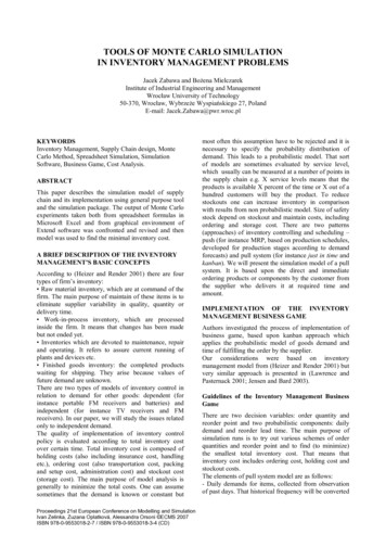
using the same principle from Glasserman (2004) wherewhereis equal in distribution to andis a standard normal distribution, we arrive at the Milstein scheme stated in Chapter 3 ofKahl and Jackel (2006) which was developed and derived by Milstein (1975)( The following substitutions from Equation (2.1), ( ))and ( ), of the Black-Scholesmodel are applied to produce the Milstein scheme for a European call option ()()Equation (3.4) is used to produce Algorithm (3.3) for the Milstein simulation of a European calloption with the initial conditions specified.1 function Milstein {2n number of paths3m number of steps4S 250 K 200 r 0.05 sigma 0.2 T 1 dt T/m;5sum 0;6for i 1 to n {7S 250;8for j 1 to m {9S S r*S*dt sigma*S*sqrt(dt)*Z 0.5*sigma 2*dt(Z 2 – 1);10}11sum sum exp(-r*T)*max(S-K,0);12}13value sum/n;14return value15 }Algorithm (3.3) A Milstein scheme simulation of a European call option.The validity of Algorithm (3.2) and (3.3) can be checked by implementing them with a comparison tothe exact Black-Scholes values. Figure (3.2) shows this overlay plot of the two schemes and that theapproximations stay in close proximity to the Black-Scholes values.15
Figure (3.2) Shows a plot of Euler and Milstein approximations to the Black-Scholes value with3.2.3 ConvergenceTo measure the accuracy of the Euler and Milstein schemes, we compare them to the solution to thestochastic equation, Equation (2.1), given by the Monte Carlo simulation. We will implement theEuler and Milstein alongside so the asset price undergoes the same variation of the random variableWith this method, we can eliminate the sampling error from the results and focus on the timestepping errors and how the two schemes differ.Consequently Algorithm (3.4) is derived from Equation (3.5) to calculate the mean absolute error ofthe Euler and Milstein schemes where both schemes use the same random variablein each timestep. The errors are calculated from the exact solution of the Monte Carlo simulation. To calculatethe mean absolute error, Equation (3.5) is used wheredenotes the number of paths,approximation and ()denotes the exact value from the Monte Carlodenotes the approximation of either the Euler or Milstein scheme.16
1 function MeanAbsoluteError {2n number of paths3m number of steps4S 250 K 200 r 0.05 sigma 0.2 T 1 dt T/m;5sum 0;6for i 1 to n {7exact SE SM 250;8for j 1 to m {9exact S*exp[(r-0.5*sigma 2)*dt sigma*sqrt(dt)*Z]10SE SE r*SE*dt sigma*S*sqrt(dt)*Z;11SM SM r*SM*dt sigma*SM*sqrt(dt)*Z 0.5*sigma 2*dt(Z 2 – 1);12}13EulerSum EulerSum abs(exact – SE)14MilsteinSum MilsteinSum abs(exact - SM)15}16EulerError EulerSum/n17MilsteinError MilsteinSum/n18return EulerError, MilsteinError19 }Algorithm (3.4) Algorithm to compute the mean absolute errors of the Euler and Milstein schemes.With the mean absolute error calculated, we look into the convergence of the errors. Seydel (2009)defines strong convergence as( )where defines the error,atwith intervals of size( ( )denotes the exact value at time ,, and)()denotes the approximationdenotes the order of convergence where. Chapter 10.2and 10.3 of Kloeden and Platen (1999) shows that the Euler scheme has a strong convergence 0.5and the Milstein scheme has a strong convergence 1.As a result we can compute the convergence order of the Euler scheme using Equation (3.6)()( )() Therefore the error of the Euler scheme can be expressed as where is the proportionality constant.17 ()
In a similar fashion, the convergence order of the Milstein scheme is also computed using Equation(3.6)()( )( )Therefore the error of the Milstein scheme can be expressed as where ()is the proportionality constant.Algorithm (3.4) is implemented and the steps are quadrupled with each simulation in the samefashion as the Monte Carlo simulation as shown in Table (3.2). Each variation of steps is repeated 3times and the mean error is calculated for both schemes.Euler ApproximationMean Er
In a growing option trading financial market, accurate option prices are necessary. There are many different approximation techniques that have been developed through the years. We look into the derivation of these models and analyse which methods are most accur