Transcription
Excel 2016Processing DataCourse objectives:1.2.3.4.Use conditional formatting effectivelyUse IF and VLOOKUP functions for data analysisUse PivotTables for flexible data presentationUse Sort and filter effectivelyStudent Training and SupportPhone:(07) 334 e PointsSt Lucia:Main desk of the Central, ARMUS and DHESL librariesHospitals:Main desk of the PACE, Herston and Mater librariesGatton:Level 2, UQ Gatton LibraryStaff Training (Bookings)Phone(07) 3365 /staffdevelopmentStaff may contact their trainer with enquiries and feedback related to training content. Please contact Staff Development for bookingenquiries or your local I.T. support for general technical enquiries.Reproduced or adapted from original content provided under CreativeCommons license by The University of Queensland Library
Table of ContentsRelative & Absolute Cell References . 4Relative cell references. 4Absolute cell references. 4Date Calculations and Conditional Formatting . 5Date calculations . 5Apply conditional formatting . 5Apply conditional formatting to a whole row . 6‘IF’ Function . 7Using ‘IF’ statements . 7Practice Exercise Basic IF Statements . 7VLookup Function . 8Using V lookup. 8Practice Exercise Vlookup . 9Pivot Table . 9Create a pivot table . 9Add data to PivotTable . 11Edit PivotTable . 11Pivot Table Slicers. 12Practice Exercise Pivot Table Exercise . 13Create a PivotChart . 14Extras Sorting & Filtering Lists . 15Sort by single criteria. 15Sort by multiple criteria. 15Filtering with AutoFilter. 16Progressive filtering . 17Find Unique Values and Remove Duplicates . 17Find unique values . 17Protection . 18Worksheet protection . 18Unprotected cells . 19Goal Seek . 19Use ‘Goal Seek’ tool . 20Naming Cells. 21Naming cells via ribbon . 21Answers . 21Exercise document:Go to ining/training-resources and click Excel. Locateand click the Processing Data.xlsx link. Make sure you are on the Relative and Absolute Referencesheet when the workbook opens.Reproduced or adapted from original content provided under CreativeCommons license by The University of Queensland Library
UQ LibraryStaff and Student I.T. Training3 of 21Ask I.T. Microsoft Excel 2013: Manipulating Data
UQ LibraryStaff and Student I.T. TrainingRelative & Absolute Cell ReferencesRelative cell referencesCalculate “% Paid”1. Select cell M22. Enter L2/K23. Press Enter4. Select cell M25. Select the % button from theNumber group on the Home tab6. Click the “Increase Decimal”button twice7. Use the Autofill tool to fill theremaining results in the column.Note: this will also carry down the % formatting.Absolute cell referencesAbsolute cell references – This uses the exact address of a cell regardless of the position ofthe cell that contains the formula.Calculate % of Total Fees Paid1. Select cell N22. Type in L2/L283. Click the % button4. Click the increase decimalsbutton5. Use the AutoFill tool to fill theremaining resultsNote: an error will display as Excel will use relative cell references by default. To correct this the dividing cellreference should be a fixed cell or an absolute reference6. Edit formula in cell N2 by doubleclicking.7. Click in L28 cell reference8. Use the function key F4 to changethe formula to an absolutereference L2/ L 28Notes4 of 21Microsoft Excel: Processing Data
UQ LibraryStaff and Student I.T. Training1. Use AutoFill to calculate theremaining resultsDate Calculations and Conditional FormattingDate calculationsDisplay hidden data1. Select column D and column F2. Right click on selection3. Select UnhideCalculate Age from Date of BirthNote: Subtracting a date of birth from the current date will display the number of days between the two dates. Tofind out the age in years, divide by 365.25 (the .25 allows for leap years).4. Select cell E25. Type in formula . ROUNDDOWN((TODAY()-D2)/365.25,0)6. Press Enter7. Use the AutoFill tool to calculate theremaining results.Note: The Rounddown function has the following structure. Rounddown(number,num digits). In the aboveformula the number portion is generated by the formula (TODAY()-d2)/365.25. The num digits portion isdesignated zero meaning all the values after the decimal round down to zero e.g. 28.96 becomes 28.00.Apply conditional formattingApply formats to students over 26 years1. Select range to be formatted:E2:E272. Select Conditional Formatting onthe Home tab3. Hover over Highlight Cell Rules4. Select Greater Than 5. Type in 266. Adjust formats to suit7. Click OKNotes5 of 21Microsoft Excel: Processing Data
UQ LibraryStaff and Student I.T. TrainingApply conditional formatting to a whole rowApply formats to students over 26 years1. Select range to be formatted:A2:N22. Select the Conditional Formatting buttonfrom the Styles group on the Home tab3. Select New Rule 4. Select “Use a formula to determine whichcells to format”5. Enter E2 26Note: This makes the column reference an absolute referencewhich means the condition will always be based on the contentof that column but on a range of rows6. Click the Format button7. Apply formatting as required8. Click OK9. Click on OK1. Select Manage Rules2. Go to the Applies To field3. Change the range to A 2: N 27Note: This will ensure the conditional formatting criteria willapply to all rows in the defined range4. Click on OKNotes6 of 21Microsoft Excel: Processing Data
UQ LibraryStaff and Student I.T. TrainingData AnalysisExcel can analyse a specified range of data using a variety of tools and can subsequentlydisplay results calculated from a formula or from user specified options‘IF’ FunctionThe IF function will analyse data and provide results defined by the user. The analysis returnseither a true or false answer. The displayed results can be text or calculated values. Averageand Final Exam grades will analyse exam results and provide a grade for students basedon pre-defined criteria.Using ‘IF’ statementsGo to the If Statement sheet1.2.3.4.Select cell D2Enter formula IF(C2 B2,C2*2%,0)Select cell E2Enter formula IF(D2 300,”Excellent”,”Poor”)5. Copy the answers down the columnsPractice Exercise Basic IF StatementsGo to the Basic If Exercise sheet.1.2.3.Follow the instructions below the tableCreate the Average (Overall Score) and IF (Final Grade) statements in their respectivecolumnsCopy the answers down the columnsSee page 21 for the answer.Notes7 of 21Microsoft Excel: Processing Data
UQ LibraryStaff and Student I.T. TrainingVLookup FunctionYou can also use the VLOOKUP function as an alternative to the IF function for elaboratetests. Lookup functions will analyse data and compare it against a predefined range prior todisplaying the result. This works on the principle:a) Here's a value.b) Go to another location and find a match for my value,c) When a match is found show the cell contents from within a specified column numberA vertical array (or table) has headings in the first row and data in column beneath. This is themost common layout for information within Excel.Note: If the Headers are in the first column and the data is in rows then you would use the HLookup function.Using V lookupUse VLOOKUP to extract data from tables of information1. Go to the “Vlookup” sheet2. Go to cell E223. Click the Insert Function button on theformula bar4.5.6.7.Type VLOOKUPClick GoSelect VLOOKUPClick OK1. Enter the Name VLOOKUP function as:1 The cell to check (Lookup value): D22 The range to compare (Table array):D4:M17 Column containing information(Col index num): 2 Exact or Approximate match(Range lookup): False (exact) Select cell F2222. Enter the Overall Score VLOOKUPfunction as: The cell to check (Lookup value): D22 The range to compare (Table array):D4:M17 Column containing information(Col index num): 10 Exact or Approximate match(Range lookup): False (exact) Select cell G2233. Enter the data opposite into the Table 1areaonthespreadsheetNotes8 of 21Microsoft Excel: Processing Data
UQ LibraryStaff and Student I.T. Training4. Enter the Final Grade VLOOKUPfunction as:4 The cell to check (Lookup value): F22 The range to compare (Table array): A4:B9 Column containing information(Col index num): 2 Exact or Approximate match(Range lookup): True (range)5. AutoFill downNote: As we are looking for an approximate match the data in column 1 of the table array A4:B9 must be sortedin ascending order.Practice Exercise VlookupGo to the VLookup Exercise sheet.1. Follow the 6 instructions at the top right2. Create a vertical lookup function toextract the name of the currency3. Create a vertical lookup function todisplay the amount of convertedcurrency.4. See page 21 for the answer.Pivot TablePivot tables allow you to extract and arrange elements of your data to present it in analternative table. With pivot tables you can group and summarise list data into a format that iseasy for reporting and analysis. A pivot table won’t automatically update if the raw datachanges and you will need to refresh to update any changes in the data.Create a pivot table1.2.3.4.Select the Fees PivotTable Data sheetClick any individual cell within the dataClick Insert tabClick Pivot Table buttonNotes9 of 21Microsoft Excel: Processing Data
UQ LibraryStaff and Student I.T. Training5. In the Create Pivot Table dialog box checkthe correct data range has been selectedand entered6. Click on New Worksheet7. Click OKA new worksheet opens8. Rename the worksheet PivotThe fields available are displayed in thePivotTable Fields List at the right of the screenNote: These are used to build the PivotTable.Pivot Table categories define 3 main areas of information:FiltersGives an overall viewwhich can be refinedColumn/Row LabelsGroups of data:e.g. Dept, Model, Product Type,Locations, SalespeopleValuesGroups of data:e.g. AmountsNotes10 of 21Microsoft Excel: Processing Data
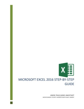
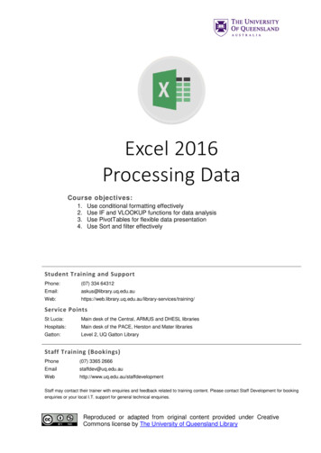
UQ LibraryStaff and Student I.T. TrainingAdd data to PivotTableTo display fees owing in each facultyDrag & Drop the following fields into the appropriatesections Year of Study into Column section Faculty into Rows section Fees Owing into Values sectionNote 1: The Report Filter allows you to apply filters to the PivotTable to display select portions only e.g. Filter by Degree TypeNote 2: The PivotTable will automatically reflect changes as youwork unless you select “Defer Layout Update.” This allows youto click the “Update” button when complete.Edit PivotTableTo rearrange the Pivot Table reposition fields asneeded.10. Drag Year of Study from Column to RowNote: The Pivot Table will adjust to display the new data layout11. Drag Year of Study above Faculty withinthe Row sectionTo change Table values displayedPivot Tables can display more than one column ofdata at a time1. Drag Faculty from the Fields List to the ValuessectionNote: Faculty as a value defaults to Count as it is text2. Drag a second Fees Owing into the Valuessection3. On the PivotTable Tools; Analyze tabClick on ‘Field Settings’ in Active Field gro
Microsoft Excel : Processing Data Add data to PivotTable To display fees owing in each faculty . Drag & Dropthe following fields into the appropriate sections Year of Study . into . Column . section Faculty. into . Rows . section Fees Owing. into . Values . section . Note 1: The Report Filter allows you to apply filters to the Pivot Table to display select portions only e.g .