WIXLIB

Dissimilarity-based compatibility We compute the dissimilarity between patches xj , xi by summing the squaredcolor difference along the abutting boundaries. For example, the left-right (LR) dissimilarity between xj , xi isDLR (xj , xi ) K X3X2(xj (k, u, l) xi (k, v, l))(5)k 1 l 1where patches xj , xi are regarded as K K 3 matrices, u indexes the last column of xj , and v indexes the firstcolumn of xi . We compute the color difference in the normalized LAB color space, where chrominance componentsare normalized to have the same variance as the luminancecomponent. We convert this squared difference to a probability by exponentiating the color difference D: D(xj , xi )(6)Pi,j (xj xi ) exp 2σc2where σc is adaptively set as the difference between thesmallest and the second smallest D(xj , xi ) among all xj .Note that the dissimilarity is not a distance: D(xj , xi ) 6 D(xi , xj ).Boosting-based compatibility We train a boosting classifier to identify matching edges by deriving a feature vectorfrom boundary pixels. Given patches xi and xj , we take a2-pixel band from each patch at the abutting boundary, andsum the squared difference of all pairwise 2-pixel bands inxi and xj . This captures the correlation between pixels atthe abutting boundary. When there are K pixels per column, the feature vector is 3 4K 2 dimensional (i.e. 3 forthe color channels). We train the classifiers using a Gentle boost algorithm [9, 19], with 35200 true samples, and35200 false samples. We use the classifier margin as thecompatibility.Set-based compatibility The set-based compatibility isinspired by the bidirectional similarity [18]. The set dissimilarity is the minimum distance between the K K patchat the abutting boundary of two patches xi , xj and all otherpatches in the database. We use the sum of squared colordifference as the distance. We exponentiate the distance asin Eq. (6) to convert it to a compatibility. Under this measure, a patch pair is compatible if their boundary region issimilar to one of the patches in the database. In our implementation, we sample the boundary region half from theleft patch and the other half from the right patch, but otherratios are possible as well.Image statistics-based compatibility Weiss and Freeman [20] present a set of filters that lies in the null spaceof natural images. We convolve the K K patch at theabutting boundary of two patches with these filters. PatchClassification accuracy3.1. Compatibility metrics0.90.80.70.60.50.40.30.20.10Dissimilarity- BoostingbasedbasedSetbasedImageCho et.al.statistics-basedTypes of compatibilityFigure 1. We evaluate five compatibility metrics based on the classification criterion. For each image in the test set consisting of20 images, we find the portion of correct patch pairs that receivedthe highest compatibility score among other candidates. We showthe average classification accuracy of 20 images. We observe thata dissimilarity-based compatibility metric is the most discriminative.pairs with a small filter response at the boundary are givena high compatibility score as in [4, 20].The compatiblity in Cho et al. [4] Cho et al. [4] combines the dissimilarity-based compatibility and the imagestatistics-based compatibility by multiplying the two.3.2. EvaluationPatch pairs that were adjacent in the original imageshould receive the highest compatibility score among others. We use this characteristic as a criterion for comparing compatibility metrics. For each patch xi , we find thematch xj with the highest compatibility, and compute forwhat fraction of test patches xi the compatibility metric assigns the highest compatibility to the correct neighbor. Weperformed this test on 20 images. Figure 1 shows the average classification accuracy for each compatibility metric.Interestingly, the naive dissimilarity-based compatibility measure outperforms other sophisticated compatibilitymeasures under the classification criterion. We can attributethis observation to the fact that the patch neighbor classification problem is that of finding the best match among theset of patches from the same image, not that of finding apatch boundary that looks as similar as possible to training images. Learning-based compatibility metrics measurehow natural the boundary regions are and do not necessarilypreserve the likeliness ranking. The compatibility metric inCho et al. [4] is useful for finding visually pleasing patchmatches other than the correct match and is useful for image editing purposes. However, for the purpose of solvingjigsaw puzzles, the dissimilarity metric is the most reliable,giving the highest classification accuracy.We also observe that the compatibility performance depends on the image content. Images with high classificationaccuracy tend to have more texture variations, whereas images with low classification accuracy lack details. To solve

the jigsaw puzzle, we use the dissimilarity-based compatibility.4. Local evidenceThe local evidence determines the image layout. Without it, the belief propagation algorithm in Section 2 generates images that do not conform to standard image layouts.In Cho et al. [4], the local evidence term at pixel i favorspatches with a similar mean RGB color as the ith pixel inthe low resolution image: (yi m(l))2p(yi xi l) exp (7)2σe2where m(l) is the mean color of patch l, i indexes pixels,and σe 0.4. In the jigsaw puzzle problem, however, wedo not have the low resolution image y.We explore two strategies to emulate a low resolutionimage: dense-and-noisy local evidence and sparse-andaccurate local evidence.4.1. A dense-and-noisy local evidenceWe estimate dense-and-noisy local evidence from a bagof image patches. We represent a bag of image patches asa patch histogram, and learn the correspondence between apatch histogram and a low resolution image.The patch histogram We create a patch vocabulary bysampling patches from training images, and clusteringthem. To have enough patches that are representative of various textures, we sample 8, 500, 000 patches of size 7 7from 15, 000 images taken from the LabelMe database [17].We explore two types of patch representations for clustering: color-based and gradient-based. The color-basedrepresentation rasterizes a patch into a 147 (7x7x3) dimensional feature vector. The gradient-based feature sums thex,y gradient of a gray-scale patch along every row and column. We augment the 28-dimensional (7x2x2) gradientbased feature with the mean RGB values, generating a 31dimensional vector. The motivation behind this representation is that similar patches tend to have similar gradientprofiles. We reduce the dimensionality of these representations to retain 98% of the original signal variance throughPrincipal Component Analysis (PCA).Clustering millions of high dimensional features is not atrivial task. We cluster the patches in two steps. First, wecluster patches sampled from the same image into L clusters. We compute the cluster center for each cluster by averaging patches that belong to the same cluster. Then were-cluster L cluster centers from all images to find the Nglobal clusters. We used the fast K-means algorithm [6] forclustering. In this paper, L 20, N 200.Given the N cluster centers, we can associate each imagewith a patch histogram h. The ith entry of a patch histogramh counts the number of patches that belong to the ith cluster. The patch histogram is fairly sparse since each imageconsists of 432 patches.The patches within boxes in Figure 2 are the 20 most occurring cluster centers when we represent patches using (a)a gradient-based feature or (b) a color-based feature. Thegradient-based feature uses the gray level and the edge information, whereas the color-based feature uses the graylevel and the color information.Properties of the patch clusters We can predict wherein the image each patch cluster is most likely to occur. Todo so, we back-project the patch cluster centers to trainingimages, and observe where in the image they occur mostfrequently. We count the number of times a patch from acertain cluster appears at each patch location. This is calledthe patch cluster probability map. The patch cluster probability maps are shown in Figure 2, pointed by the arrowsfrom the corresponding cluster centers.Probability maps of the gradient-based patch representation show that clusters corresponding to edges tend to bein the foreground, but do not have strong spatial constraints.The clusters encoding intensity information carry more spatial information: bright patches usually appear at the topsince objects near the sky (or the sky itself) are brighter thanother objects in the scene.The clusters from the color-based patch representationcapture both intensity and color information. The patchprobability maps show that some colors correspond to natural lighting, background scenes, or vignetting effects, andsome other colors correspond to foreground objects. For example, a blue patch predominantly occurs in the upper halfof the image, whereas brown and dark red colors most frequently correspond to foreground objects. The patch mapsshow a rich set of location constraints for different patchclasses. (We anticipate that other feature representations,such as SIFT, would show similarly rich spatial localizationstructure.) This structure allows us to very roughly placeeach feature in the image, or to estimate a low-resolutionimage from the bag of features.A probability map can be used as a patch prior. If a cluster s appears often at node i, patches that belong to the cluster s are given higher probability to appear at node i.Image estimation through regression We learn a linearregression function A that maps the patch histogram h to thelow resolution image y, training A on images that were alsoused to find cluster centers. We use the color-based patchrepresentation since it captures more spatial information.Let columns of H be the patch histograms of trainingimages, and columns of Y be the corresponding low resolution images. We learn the regression function A as follows[1]:A Y H T (HH T ) 1(8)

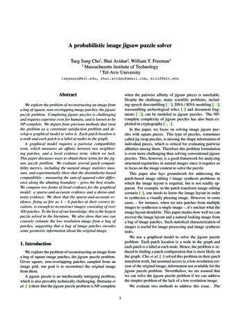
probability map scalePatch cluster probability mapsmax/2maxPatch clusters0(a) Gradient based feature(b) Color based featureFigure 2. The patches in rectangular boxes are the top 20 most occurring patch cluster centers when we use (a) a gradient-based / (b) acolor-based representation. Around the boxes are patch probability maps for a subset of cluster centers, pointed by the arrows from thecorresponding patch cluster.Estimatedlow-res imagePatch histogramThe number of entries from the imageInput imageCorrectpatch 80200160180200160180200160180200The number of entries from the imageThe cluster number16014012010080604020020406080100120140The number of entries from the imageThe cluster number605040302010020406080100120140The number of entries from the imageThe cluster number100908070605040302010020406080100120140The cluster numberRanking map scaleFirstLastFigure 3. The patch histogram can be used to estimate a low resolution image. The regression function generates a low resolutionimage that resembles the original image, but we can nonethelessfind examples that fail (the last row). The last column is a patchrank map: At each node, we order patches based on the likelihoodgiven the estimated low resolution image, and show the rank of thetrue patch. Most of the correct patch rankings score high using theregression function – the ideal result is deep blue everywhere.The size of the original image is roughly 700 500, and theestimated low resolution image is 24 18.Figure 3 shows some experimental results. We observethat the regression can coarsely predict the low resolutionimage. This observation counters the intuition that the bagof features does not encode any spatial information. Onepossible explanation is that there are enough structural regularities in images so that a bag of features implicitly captures the geometric information. For example, when thereare many patches that belong to a blue cluster, it’s likely thatthey constitute a blue sky. Of course, it is easy to find failure examples: the blue tone of snow is misclassified as skyin the last example in Figure 3. Nevertheless, the regression function learns important image regularities: something bright should be at the top, illuminating foregroundobjects at the bottom.We quantitatively evaluate the accuracy of the estimatedlow resolution image using a patch rank map. At each node,we order patches based on the likelihood given the estimated low resolution image, and show the rank of the truepatch. Ideally, we want the true patch to have rank 1 at allnodes. We observe from the last column in Figure 3 that thepatch rank is quite low in most nodes, except for nodes thatcorrespond to foreground objects or the transition betweenthe background and the foreground. On average (acrossall nodes and across 20 test images), the true patch has arank 151 among 432 patches. We used the linear regression model because the kernel regression did not noticeablyimprove the quality of estimated low resolution images, yetrequired much more computation.4.2. A sparse-and-accurate local evidenceWe explore another strategy to emulate the low resolution image in Eq. (7). We study a scenario where somepatches are associated with the correct positions in the puzzle. We name these patches the anchor patches. This is ageneralization of the puzzle solving strategy that first fixesthe four corner pieces and works its way inward. We showthat the puzzle solver accuracy improves as we add moreanchor patches and as the anchor patches are spread out uniformly across the image.5. Solving the jigsaw puzzleWe reconstruct the jigsaw puzzle by maximizing p(x)(Eq. (1)) using loopy belief propagation [4]. Since loopybelief propagation can fall into a local minimum, we run

Reconstruction accuracyOriginal imageDirect comparisonCluster comparisonNeighbor comparison0.8Reconstructed e numberFigure 4. The image reconstruction accuracy with the estimatedlow resolution image for 20 different test images.loopy belief propagation three times with random seeds andpick the best reconstruction in terms of the reconstructionaccuracy. Each image is broken into 432 patches of size 28x 28, which is down-sampled to 7 x 7 for low resolutionimage estimation.Performance metrics While there has been an extensivework on solving jigsaw puzzles, there has not been any measure that evaluates the puzzle reconstruction performancebecause the previous works treated the puzzle solving as abinary problem. We propose three measures that gauge partial puzzle reconstruction performance: Direct comparison: the inferred patch labels are compared directly to the ground-truth patch labels. The reconstruction accuracy measures the fraction of nodesfor which the algorithm inferred the correct patch. Cluster comparison: the inferred patch labels aremapped to clusters they belong to, and are comparedto the ground-truth cluster labels. The reconstructionaccuracy measures the fraction of nodes for which thealgorithm inferred the correct cluster. Neighbor comparison: for each assigned patch label,we compute the fraction of four neighbor nodes thatthe algorithm assigned the correct patch (i.e. patchesthat were adjacent in the original image). The reconstruction accuracy is the average fraction of correctneighbor labels.The direct comparison measure penalizes all patches thatare assigned to wrong nodes, but the cluster comparisonmeasure tolerates the assignment error as long as the assigned patch belong to the same cluster as the ground-truthpatch. The neighbor comparison measure does not careabout the exact patch assignment as long as patches thatwere adjacent in the original image remain adjacent.(b)Figure 5. Two examples ((a) image 8, (b) image 20) of reconstructed images using the estimated local evidence.5.1. Reconstruction with dense-and-noisy local evidenceWe use the estimated low resolution image and the patchprior to solve the puzzle. The reconstruction accuracy for 20test images is shown in Figure 4. Clearly, the graph suggeststhat it is hard to reconstruct the original image even giventhe estimated low resolution image.To better understand Figure 4, we show two image reconstructions in Figure 5. The overall structure of reconstructed images is similar to that of the original images.Also, while parts of the image are not reconstructed properly, some regions are correctly assembled even though theymay be offset from the correct position. The tower in Figure 5 (a) and the car road Figure 5 (b) have been laterallyshifted. This can be attributed to the fact that the estimatedlow resolution image does not provide enough lateral information. Such shifts in image regions are not tolerated by thedirect comparison measure and, possibly, the cluster comparison measure, but the neighbor comparison measure ismore generous in this regard. In fact, under the neighborcomparison measure, the average reconstruction accuracyis nearly 55%, suggesting that many regions are assembledcorrectly but are slightly shifted.5.2. Reconstruction with sparse-and-accurate localevidenceWe study the jigsaw puzzle reconstruction performancewith a sparse-and-accurate local evidence. In particular, wewant to study how the number of anchor patches affect theimage reconstruction accuracy. We run the image reconstruction experiments for 0 to 10 anchor patches.Figure 6 illustrates that the location of anchor patchesmatters as well as the total number of anchor patches. If theanchor patches are more spread out, the image reconstruction performance improves. Therefore, we predefined the

(a)(b)Original imageIncreasing the number of anchor patchesFigure 7. This figures shows two examples of reconstructed images with a sparse-and-accurate local evidence. As we increase the numberof anchor patches (shown red), the algorithm’s performance improves.under all reconstruction measures. This is because the estimated low resolution image is too noisy.5.3. Solving a smaller jigsaw puzzleFigure 6. To improve the reconstruction accuracy, it’s better tospread out the anchor patches (red) evenly across the image.location of anchor patches such that they cover the image asuniformly as possible. This has an important consequencethat even if we do not have anchor patches, we can loop over432patch combinations to find the correct anchor patcheskat k predefined nodes. Figure 7 shows some image reconstruction results (see supplemental materials for more examples).Figure 8(a) shows the reconstruction accuracy, averagedover the 20 test images. As expected, the average accuracy improves as we increase the number of anchor patches.Anchor patches serve as the local evidence for neighboringimage nodes. As we add more anchor patches, more nodesbecome closer to anchor patches, and thus more nodes canreliably infer the correct patch label.To calibrate the performance of the sparse-and-accuratelocal evidence scheme, we run another set of experimentswith a quantized 6-bit true low resolution image. The reconstruction accuracy is overlaid on Figure 8. The performance of using a 6-bit true low resolution image is comparable to using 6 10 anchor patches. This also suggeststhat solving the puzzle with the estimated low resolution image is extremely challenging. The estimated low resolutionimage should be as accurate as a 6-bit true low resolutionimage in order to perform comparably to using the sparseand-accurate local evidence.We also compared the performance of using the sparseand-accurate local evidence to using a combination of anchor patches and the estimated low resolution image. Thereconstruction performance is shown with dotted lines inFigure 8(a). When there are no anchor patches, the estimated low resolution image helps better reconstruct theoriginal image. However, as we introduce anchor patches,on average, it is better not to have any noisy local evidenceWe have performed the same set of experiments on asmaller jigsaw puzzle. Each small jigsaw puzzle consists of221 pieces. Figure 8(b) shows the reconstruction accuracy.The figure shows that we need fewer anchor patches to almost perfectly reconstruct images. In fact, we can perfectlyreconstruct 5 images, and the top 15 images have the reconstruction accuracy higher than 90% under the most stringentdirect comparison measure. A few images are difficult to reconstruct because they contain a large, uniform region.6. ConclusionWe introduce a probabilistic approach to solving jigsawpuzzles. A puzzle is represented as a graphical model whereeach node corresponds to a patch location and each labelcorresponds to a patch. We use loo

a bag of image patches. Such statistical characterization of images is useful for image processing and image synthesis tasks. We use a graphical model to solve the jigsaw puzzle problem: Each patch location is a node in the graph and each patch is a label at each node. Hence, the problem is re-