WIXLIB

smoothing using a naı̈ve spline algorithm. After the preprocessing step, the piece fitting andlocking algorithms were run until completion. Unlike most previous puzzle solving algorithms,ours work from the “inside out”; in other words, the initially selected piece tends to belocated inside the puzzle, not on its boundary, and the subsequent pieces are successivelyfitted together, building the puzzle up from its interior, and avoiding any need to identifyboundary pieces as such. With appropriate choices of adjustable parameters, effectivelybalancing processing speed versus accuracy of the piece placements, the Rainforest and Bafflerpuzzles were successfully solved in, respectively, 58 and 31 minutes on an Intel R CoreTM 2Duo E8500 3.17GHz processor.The final section presents some preliminary investigations into scalability of our algorithmto even larger puzzles. The Cathedral jigsaw puzzle [29], is a non-standard 1000 piece puzzle,yet its individual pieces contain many standard “indents” and “outdents.” This combinationmakes it particularly challenging, since there are many “local” near-matches, and yet simplified algorithms designed for standard puzzles cannot be applied because of the unusualstructure. While we have not, as yet, achieved complete success in this much more challenging situation, the algorithm did successfully assemble 103 pieces of a 111 piece subpuzzlebefore terminating, in approximately 36 hours. If we had a similar sized puzzle with moreirregular pieces, as in the Baffler, we would expect much greater success. Thus, while furtherwork remains to be done, our conclusion is that the algorithm does lend itself to applicabilityto much larger puzzles and is eminently scalable.2Curves and Puzzles.Let us introduce our basic terminology and assumptions, based on that used in [15, 16]. Wewill be working exclusively with plane puzzles. (Extending our methods to three-dimensionalpuzzles, e.g., a broken statue, would be an interesting challenge. While the mathematicalmachinery is in place, [20], their practical implementation remainspdaunting.) We will workin the Euclidean plane with the standard norm, denoted k z k x2 y 2 for z (x, y) R 2 . We let SE(2) denote the three-dimensional special Euclidean group consisting of allorientation-preserving isometries, or rigid motions: xcos θ sin θa2z 7 R z c, z R , where R , c , (2.1)ysin θcos θbare, respectively, a 2 2 matrix representing rotation through angle θ and a translationvector. We will consistently identify planar objects up to rigid motion. All curves C R 2are assumed to be compact, rectifiable — and hence of finite length — and simple, i.e.,without self-intersections. A closed curve is called a Jordan curve, while a non-closed curve,with distinct endpoints, will be called an arc. Two arcs are said to be non-overlapping if theyhave at most one or both endpoints in common.By definition, a puzzle piece is a bounded, simply connected plane domain P R 2 whosee are congruent, andboundary C P is a Jordan curve of class C3 . Two puzzle pieces P, Phence considered to be the same, if they are rigidly equivalent, meaning that there is a rigide g · P. Two puzzle pieces P, Pe are said to fit together if theymotion g SE(2) such that Pe P P,e or, more generally, if they do so after a rigidshare a common arc S P P4

e (g · P) Pe (g · P) for some g SE(2). Keep in mind that pieces that fitmotion: S Pdo not overlap. In practice, the shared arc should not be too short, although this requirementneed not be directly quantified as it will follow as a consequence of our fitting and lockingalgorithms. We can also allow two puzzle pieces to fit along more than one connected arc,although this is uncommon in real world puzzles. It is also not difficult to allow non-simplyconnected puzzle pieces, again rare in examples.Remark: The key assumption used in this work is that the puzzle pieces are smooth (ofclass C3 ), and hence do not have corners. Clearly, many physical puzzles contain pieces withcorners, and it would be worth directly adapting our algorithms to cover such pieces. Suchan extension will not be difficult; indeed, during the course of the assembly process, we dealwith subpuzzles, that is, unions of puzzle pieces, whose boundary is only piecewise C3 (andnot necessarily simply connected). However, this adaption has proven to be unnecessary forthe practical solution of all the puzzles we have tried, since the digital images of the puzzlepieces must be subjected to a preliminary smoothing operation anyways before the assemblyalgorithm can proceed.By an apictorial puzzle, or puzzle for short, we mean a bounded plane domain P R 2that is the union,n[P (gi · Pi ),(2.2)i 1of individual puzzle pieces Pi subject to rigid motions gi SE(2), which we sometimesrefer to as placements. We suppose that any two pieces, when placed, are either disjoint,(gi · Pi ) (gj · Pj ) , or touch at a single point1 { z0 } (gi · Pi ) (gj · Pj ), or fit togetheraccording to the preceding definition. However, while standard jigsaw puzzles satisfy this,our algorithms don’t actually require this assumption to hold, and so could, in principle,solve “multi-layered puzzles”, whose pieces are allowed to overlap. (While this strikes us asan intriguing extension of standard jigsaw puzzles, we are not aware of any actual examples.)In the puzzle assembly problem, we are given the pieces P {P1 , . . . , Pn }, and our task is todetermine the corresponding rigid motions g1 , . . . , gn required to assemble P. Our methodswork best when pieces that fit together do so uniquely, and only fit in accordance with theirpositions in the final puzzle assembly. However, more sophisticated backtracking techniquescould be developed to better deal with non-uniqueness of fits (e.g., as in [18]).3Equivalence of Curves.Our algorithm for fitting puzzle pieces together is based on the solution to the equivalenceproblem for plane curves based on extended Euclidean-invariant signatures developed in [16].Let us review the key points, leaving the complete details to the aforementioned reference.Given a C3 Jordan curve C R 2 , let z(s), 0 s L, denote its arc length parametrization, so that L is the length of C and z(s) is periodic of period L. Let κ(s) denote thesigned curvature at the point z(s) C, and κs (s) dκ/ds its derivative with respect to arc1More generally, one can allow pieces to touch at a finite number of points, although this is uncommonin real world examples.5

length. Note that both κ and κs are Euclidean differential invariants, meaning that they areunaffected by rigid motions, [20].A point z(s) C is called regular if κs (s) 6 0. An ordinary vertex is a local extremumof curvature, [15]. We define a generalized vertex to be maximal connected arc V C onwhich κs (s) 0. Thus, a generalized vertex is either an ordinary vertex, or a critical point ofcurvature, or a circular arc, or a straight line segment. In this paper, all curves are assumedto be v-regular, [16], meaning that they have only finitely many generalized vertices. Curveswith infinitely many vertices exist in theory, but are pathological and cannot arise in realworld applications.By a bivertex arc, we mean an arc B C that has κs 0 at both endpoints, but all ofwhose interior points are regular. A basic result of [16] states any v-regular C3 Jordan curvethat is not a circle has a unique bivertex decomposition,C m[Bj j 1n[Vk ,(3.1)k 1into a finite union of m 4 non-overlapping bivertex arcs B1 , . . . , Bm , and n 0 generalizedvertices V1 , . . . , Vn . Note that we exclude point vertices from the bivertex decomposition,since they are accounted for by the endpoints of the bivertex arcs Bj .e R 2 are said to be rigidly equivalent, or congruent for short, ifTwo plane curves C, Ce g·C. We extend the notion of congruencethere exists a rigid motion g SE(2) such that Cto disconnected unions of curves, keeping in mind that for two unions to be congruent, theirconstituent curves must be pair-wise congruent under the same rigid motion. The followingresult was established in [16].e R 2 are congruent if and only if theProposition 1. Two v-regular plane curves C, Cunions of their constituent bivertex arcs are congruent.Using a reformulation of Cartan’s general solution to the local equivalence problem ofsubmanifolds under Lie group actions, [5], a solution to the equivalence problem for planecurves based on their Euclidean signature was proposed in [4], and subsequently applied toobject recognition and symmetry detection in a variety of contexts, [25, 26].Definition 2. Let C be a plane curve of class C3 and of length L . The Euclidean signature of C is the (non-simple) plane curve S(C) { (κ(s), κs (s)) 0 s L } parametrizedby the curvature and its derivative with respect to arc-length.The following theorem is a consequence of Proposition 1, combined with general resultson group-invariant signatures2 of regular submanifolds, [20].e R 2 be v-regular, non-circular Jordan curves whose bivertex decomTheorem 3. Let C, Cpositions contain the same number, n, of non-overlapping bivertex arcs. Assume that, forej have identical signatures: S(Bj ) S(Bej ),each j 1, . . . , n, the bivertex arcs Bj and Bej are congruent, and hence there exist rigid motions gj SE(2) suchwhich implies that Bj , Bej gj · Bj . If, in addition, all the gj g are the same, then the entire curves arethat Be g · C.rigidly equivalent: C2The older term “classifying submanifold” is used in place of “signature” in [20].6

In practical applications, the puzzle pieces are inputted to the computer as digital imagesand then segmented to retrieve their boundaries. (See Section 6 for practical details.) Asa result, each piece is represented by a discrete set of sample points C {z 1 , . . . , z N },where each z j lies on or near its boundary curve C. The actual curve can be approximatelyreconstructed from C by some form of interpolation, e.g., periodic splines, possibly coupledwith smoothing to reduce the effect of noise. We similarly (approximately) discretize thesignature curve S(C) by S (σ 1 , . . . , σ N ), where each point σ j (κj , κjs ) S consistsof suitable numerical approximations to the curvature and its arc length derivative at thecorresponding sample point z j (xj , y j ) C . For example, the entries of σ j may befound directly from the discretized curve C by employing the Euclidean-invariant numericalapproximations to the curvature invariants developed in [1, 4].According to the algorithm developed in [16], to determine if two discretized curves arerigidly equivalent, the first step is to construct their (approximate) bivertex decompositionsby splitting each curve into subarcs whenever κs δ0 changes sign, where δ0 0 is a fixedsmall cut-off. In order to achieve more consistent approximate Bivertex Arc Decompositions,we additionally split curves wherever κs achieves a local minimum, provided that minimumexceeds the parameter δ0 . This added convention helps to reduce sensitivity to the valueof δ0 . Additionally, instead of eliminating insignificant arcs over which curvature changesby less than δ1 (as in [16]), we eliminate arcs on which the maximum of κ is less than δ1 .Details on the selection of δ0 and δ1 are presented in [16], though we note that in this papere therein is taken as a maximum over all inputed pieces (rather thanthe quantity Dκ (C, C)just two), and is denoted dκ .The next step is to compare individual (discrete) bivertex arcs using their (discrete) Euclidean signatures. The method, developed in detail in [16], is based, roughly, on the idea ofregarding the discrete signatures as two collections of oppositely charged points, and determining the mutual electrostatic attraction, [31]. (Or, equivalently, their mutual gravitationalattraction as point masses.) After some manipulation, we determine a signature similaritye [ 0, 1 ] that serves to measure the closeness of two individual bivertex arccoefficient p(B, B)e decreases to 0 as thesignatures, where a score of 1 reflects identical signatures, while p(B, B)signatures become increasingly disparate, and hence the arcs less and less likely to be congruent. To compare the two curves, we first construct approximate bivertex decompositions,and then ensure that they contain the same number of arcs; if not, there is a good chance thecurves are not rigidly equivalent, but this may be due to noise, even with our selection of thecut-off parameter δ0 . In this case, the procedure for eliminating arcs from the larger collectionis to delete those on which the curvature changes least. Sometimes, several possible deletionsare tested. We then test the pairwise congruence of the resulting two collections of bivertexarcs, ordered as one traverses the curves with the same orientation. If they are congruent,one then checks whether the corresponding rigid motions are (approximately) identical, andif so the curves are deemed to be congruent.4Puzzle Assembly.We now present the steps used in our puzzle solving algorithm. The method relies on successively fitting individual pieces by matching bivertex arcs along their boundaries and then7

improving the fits via piece locking. The details of piece fitting and locking will appear inthe following section.We begin with the collection of puzzle pieces, denoted P {P1 , . . . , Pn }, whose boundaries Cj Pj are supplied as suitably segmented and smoothed (discrete) plane curves.The puzzle is solved by constructing a corresponding collection of rigid motions G {g1 , . . . , gn } SE(2) that form the completed puzzle (2.2). Without loss of generality,one of these can be fixed as the identity transformation: gi1 e.At each step k 1, 2, . . . , in the algorithm, we will have already assembled a subpuzzleQk P consisting of k pieces Q k { Pi1 , . . . , Pik } P , along with the corresponding rigidmotions Hk { gi1 , . . . , gik } required to assemble it:Qk k[(giν · Piν ) P.(4.1)ν 1Let R k P \ Q k denote the set of pieces that remain to be assembled. The algorithmterminates with either a fully assembled puzzle, with Qn P, or, for some k n, a subpuzzleQk ( P, for which the program is unable to fit any of the pieces remaining in R k .For each 1 j n, we let Bj {B1 , . . . , Bmj } be the set of bivertex arcs (or, moreaccurately, discrete approximate bivertex arcs) associated with the puzzle piece Pj . It willbe important to order the arcs in Bj consecutively as the boundary Cj is traversed in acounterclockwise manner. During the assembly process, any bivertex arcs that have alreadybeen fit to neighboring pieces, after successful piece locking, are deemed to be inactive, andso not available during the subsequent fitting process. We letVk k[Bi νν 1denote the set of active bivertex arcs for the subpuzzle Qk . In principle, Vk should onlycontain the bivertex arcs situated on the outer boundary of Qk , although noise or otherartifacts might prevent some interior bivertex arcs from being matched and hence remainingin Vk by “accident”. Fortunately, this does not seriously affect the performance of ouralgorithm in practical situations.It should be noted that for the purposes of pairing bivertex arcs, each assembled pieceretains its individuality, and bivertex arcs on a piece boundary remain consecutive whetheror not they are currently active. One evident limitation is that the program doesn’t considercombinations of, say, two bivertex arcs from one assembled piece and three from an adjacentassembled piece, fitting five consecutive arcs on a not yet placed piece. On the other hand,the algorithm does use this extra information during piece locking, when the assembled subpuzzle is treated as a single piece. While developing a way to universally treat subpuzzles assingle pieces could improve performance, it seemed unnecessary for many practical situations,including the puzzles treated here.The first step in the assembly algorithm is to select a piece to form the initial subpuzzle Q1 { Pi1 }, and, by default, set gi1 e. The choice of starting piece is notP so important.Our convention is to choose the piece that maximizes the total curvature κi , summedover all the points in the piece’s discretized signature, because, as argued in [16], arcs of8

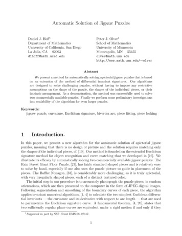
high curvature tend to “better” determine a simple closed curve. Our aim is to maximizethe chances of finding successful fits early on, by ensuring that the starting piece has manywell-defined features. Indeed, since straight lines are of minimal curvature — and also notincluded in the bivertex arcs and not candidates for fitting — this initial selection is alsomore likely to be an interior piece of the puzzle.To continue, at each step k 1, we construct the next subpuzzle by finding an unattachedpiece Pi R k that fits the current subpuzzle Qk under a rigid motion gi SE(2), and G { g }. We select the piece P through anthen setting Q k 1 Q k { Pi }, Gk 1iikadaptation of the piece fitting and locking algorithms; details appear in the following section.If no suitable piece can be found, the algorithm terminates. Otherwise, the bivertex arcs thatwere deemed to be matched in the piece locking stage that attaches Pi to Qk are relabeledas inactive, and hence deleted from the collection Vk Bi in order to form the new set of .active bivertex arcs Vk 1Remark: A more sophisticated approach would be to allow several distinct subpuzzles tobe assembled concurrently, and then deal with the problem of fitting the subpuzzles together.This proved to be not necessary for the puzzles we tried our algorithm on.5Fitting Puzzle Pieces Together.In this section, we present our algorithms for fitting and locking two individual puzzle pieces.At the end, we explain how to adapt the basic algorithms to fit and lock a piece with asubpuzzle.e by a fit, we just mean a rigid motion g SE(2).As above, given two puzzle pieces P, P,e FindingThe quality of the fit g measures how well an arc of g · C approximates an arc of C.a good fit is accomplished in two steps. First, we apply the extended Euclidean-invariantsignature method developed in [16] to form a stockpile of potential piece-to-piece fits. Fitse confidence scores. We then attempt to refine the fitsare ranked according to their µ(P, P)using the ensuing method of piece-locking. Once a lock of sufficiently high quality is found,that piece is added to the subpuzzle.We remark that an algorithm that relies solely on selecting fits with the highest confidencescores, without the extra refinement of piece-locking, is reasonably successful at solving smallpuzzles. However, the resulting fit transformations tend to be insufficiently accurate, andthe method can easily accumulate increasing errors that can hinder its success with largerpuzzles. Figure 1(a), for instance, shows such a solution of a nine puzzle piece fragment.While the pieces have been placed with correct adjacency, it is clear from figure 1(b) thatthe refinement provided by piece locking generates a much better solution.This may well inspire the reader to ask why not proceed directly to piece locking andavoid the preliminary signature-based fitting procedure? The reason is efficiency: directpiece-locking method is much slower than signature comparison, especially as the curvatureinvariants comprising the signature were already been computed in order to characterize therequired bivertex arcs. Our combination of preliminary fitting followed by the more accuratelocking procedure on potential fits appears optimal for both speed and reliability.9

(a) Solution by fit finding only(b) Solution by fit finding and piece lockingFigure 1: Two solutions of a nine piece puzzle fragment. Each has correct adjacency, but (b)improves on (a) through the

puzzles. While of limited practical use, at least outside the entertainment world, puzzle assembly has been studied with a number of more important applications in mind. In [18, 24], for instance, puzzle solution techniques are applied to broken tiles to